from keras.datasets import boston_housing
(train_data,train_targets),(test_data,test_targets) = boston_housing.load_data()
Downloading data from https://storage.googleapis.com/tensorflow/tf-keras-datasets/boston_housing.npz
57344/57026 [==============================] - 0s 3us/step
train_data.shape
(404, 13)
test_data.shape
(102, 13)
train_targets
array([15.2, 42.3, 50. , 21.1, 17.7, 18.5, 11.3, 15.6, 15.6, 14.4, 12.1,
       17.9, 23.1, 19.9, 15.7,  8.8, 50. , 22.5, 24.1, 27.5, 10.9, 30.8,
       32.9, 24. , 18.5, 13.3, 22.9, 34.7, 16.6, 17.5, 22.3, 16.1, 14.9,
       23.1, 34.9, 25. , 13.9, 13.1, 20.4, 20. , 15.2, 24.7, 22.2, 16.7,
       12.7, 15.6, 18.4, 21. , 30.1, 15.1, 18.7,  9.6, 31.5, 24.8, 19.1,
       22. , 14.5, 11. , 32. , 29.4, 20.3, 24.4, 14.6, 19.5, 14.1, 14.3,
       15.6, 10.5,  6.3, 19.3, 19.3, 13.4, 36.4, 17.8, 13.5, 16.5,  8.3,
       14.3, 16. , 13.4, 28.6, 43.5, 20.2, 22. , 23. , 20.7, 12.5, 48.5,
       14.6, 13.4, 23.7, 50. , 21.7, 39.8, 38.7, 22.2, 34.9, 22.5, 31.1,
       28.7, 46. , 41.7, 21. , 26.6, 15. , 24.4, 13.3, 21.2, 11.7, 21.7,
       19.4, 50. , 22.8, 19.7, 24.7, 36.2, 14.2, 18.9, 18.3, 20.6, 24.6,
       18.2,  8.7, 44. , 10.4, 13.2, 21.2, 37. , 30.7, 22.9, 20. , 19.3,
       31.7, 32. , 23.1, 18.8, 10.9, 50. , 19.6,  5. , 14.4, 19.8, 13.8,
       19.6, 23.9, 24.5, 25. , 19.9, 17.2, 24.6, 13.5, 26.6, 21.4, 11.9,
       22.6, 19.6,  8.5, 23.7, 23.1, 22.4, 20.5, 23.6, 18.4, 35.2, 23.1,
       27.9, 20.6, 23.7, 28. , 13.6, 27.1, 23.6, 20.6, 18.2, 21.7, 17.1,
        8.4, 25.3, 13.8, 22.2, 18.4, 20.7, 31.6, 30.5, 20.3,  8.8, 19.2,
       19.4, 23.1, 23. , 14.8, 48.8, 22.6, 33.4, 21.1, 13.6, 32.2, 13.1,
       23.4, 18.9, 23.9, 11.8, 23.3, 22.8, 19.6, 16.7, 13.4, 22.2, 20.4,
       21.8, 26.4, 14.9, 24.1, 23.8, 12.3, 29.1, 21. , 19.5, 23.3, 23.8,
       17.8, 11.5, 21.7, 19.9, 25. , 33.4, 28.5, 21.4, 24.3, 27.5, 33.1,
       16.2, 23.3, 48.3, 22.9, 22.8, 13.1, 12.7, 22.6, 15. , 15.3, 10.5,
       24. , 18.5, 21.7, 19.5, 33.2, 23.2,  5. , 19.1, 12.7, 22.3, 10.2,
       13.9, 16.3, 17. , 20.1, 29.9, 17.2, 37.3, 45.4, 17.8, 23.2, 29. ,
       22. , 18. , 17.4, 34.6, 20.1, 25. , 15.6, 24.8, 28.2, 21.2, 21.4,
       23.8, 31. , 26.2, 17.4, 37.9, 17.5, 20. ,  8.3, 23.9,  8.4, 13.8,
        7.2, 11.7, 17.1, 21.6, 50. , 16.1, 20.4, 20.6, 21.4, 20.6, 36.5,
        8.5, 24.8, 10.8, 21.9, 17.3, 18.9, 36.2, 14.9, 18.2, 33.3, 21.8,
       19.7, 31.6, 24.8, 19.4, 22.8,  7.5, 44.8, 16.8, 18.7, 50. , 50. ,
       19.5, 20.1, 50. , 17.2, 20.8, 19.3, 41.3, 20.4, 20.5, 13.8, 16.5,
       23.9, 20.6, 31.5, 23.3, 16.8, 14. , 33.8, 36.1, 12.8, 18.3, 18.7,
       19.1, 29. , 30.1, 50. , 50. , 22. , 11.9, 37.6, 50. , 22.7, 20.8,
       23.5, 27.9, 50. , 19.3, 23.9, 22.6, 15.2, 21.7, 19.2, 43.8, 20.3,
       33.2, 19.9, 22.5, 32.7, 22. , 17.1, 19. , 15. , 16.1, 25.1, 23.7,
       28.7, 37.2, 22.6, 16.4, 25. , 29.8, 22.1, 17.4, 18.1, 30.3, 17.5,
       24.7, 12.6, 26.5, 28.7, 13.3, 10.4, 24.4, 23. , 20. , 17.8,  7. ,
       11.8, 24.4, 13.8, 19.4, 25.2, 19.4, 19.4, 29.1])
mean = train_data.mean(axis=0)
train_data -= mean
std = train_data.std(axis=0)
train_data /= std
test_data -= mean
test_data /= std
from keras import models
from keras import layers
def build_model():
model = models.Sequential()
model.add(layers.Dense(64,activation='relu',input_shape=(train_data.shape[1],)))
model.add(layers.Dense(64,activation='relu'))
model.add(layers.Dense(1))
model.compile(optimizer='rmsprop',loss='mse',metrics=['mae'])
return model
import numpy as np
k = 4
num_val_samples = len(train_data) // k
num_epochs = 100
all_scores = []
for i in range(k):
print('processing fold #',i)
val_data = train_data[i*num_val_samples:(i+1)*num_val_samples]
val_targets = train_targets[i*num_val_samples:(i+1)*num_val_samples]
partial_train_data = np.concatenate(
[train_data[:i*num_val_samples],
train_data[(i+1)*num_val_samples:]],
axis=0)
partial_train_targets = np.concatenate(
[train_targets[:i*num_val_samples],
train_targets[(i+1)*num_val_samples:]],
axis=0)
model = build_model()
model.fit(partial_train_data,partial_train_targets,
epochs=num_epochs,batch_size=1,verbose=0)
val_mse,val_mae = model.evaluate(val_data,val_targets,verbose=0)
all_scores.append(val_mae)
processing fold
processing fold
processing fold
processing fold
all_scores
[2.2075135707855225, 2.5066304206848145, 2.6380698680877686, 2.472360610961914]
np.mean(all_scores)
2.456143617630005
num_epochs = 500
all_mae_histories = []
for i in range(k):
print('processing fold #',i)
val_data = train_data[i*num_val_samples:(i+1)*num_val_samples]
val_targets = train_targets[i*num_val_samples:(i+1)*num_val_samples]
partial_train_data = np.concatenate(
[train_data[:i*num_val_samples],
train_data[(i+1)*num_val_samples:]],
axis=0)
partial_train_targets = np.concatenate(
[train_targets[:i*num_val_samples],
train_targets[(i+1)*num_val_samples:]],
axis=0)
model = build_model()
history = model.fit(partial_train_data,partial_train_targets,
validation_data = (val_data,val_targets),
epochs=num_epochs,batch_size=1,verbose=0)
mae_history = history.history['val_mae']
all_mae_histories.append(mae_history)
processing fold
<tensorflow.python.keras.callbacks.History object at 0x00000158F12E0EE0>
processing fold
<tensorflow.python.keras.callbacks.History object at 0x00000158F0D80070>
processing fold
<tensorflow.python.keras.callbacks.History object at 0x00000158EF0C7B50>
processing fold
<tensorflow.python.keras.callbacks.History object at 0x00000158F0B9DB20>
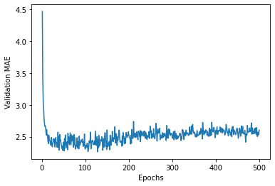
average_mae_history = [
np.mean([x[i] for x in all_mae_histories]) for i in range(num_epochs)
]
import matplotlib.pyplot as plt
plt.plot(range(1,len(average_mae_history) + 1),average_mae_history)
plt.xlabel('Epochs')
plt.ylabel('Validation MAE')
plt.show()
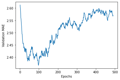
def smooth_curve(points, factor=0.9):
smoothed_points = []
for point in points:
if smoothed_points:
previous = smoothed_points[-1]
smoothed_points.append(previous * factor + point*(1-factor))
else:
smoothed_points.append(point)
return smoothed_points
smooth_mae_history = smooth_curve(average_mae_history[10:])
plt.plot(range(1,len(smooth_mae_history) + 1),smooth_mae_history)
plt.xlabel('Epochs')
plt.ylabel('Validation MAE')
plt.show()
model = build_model()
model.fit(train_data,train_targets,epochs = 80,batch_size=16,verbose=0)
test_mse_score,test_mae_score = model.evaluate(test_data,test_targets)
4/4 [==============================] - 0s 2ms/step - loss: 18.2394 - mae: 2.6816
test_mae_score
2.6815996170043945


【推荐】国内首个AI IDE,深度理解中文开发场景,立即下载体验Trae
【推荐】编程新体验,更懂你的AI,立即体验豆包MarsCode编程助手
【推荐】抖音旗下AI助手豆包,你的智能百科全书,全免费不限次数
【推荐】轻量又高性能的 SSH 工具 IShell:AI 加持,快人一步