clusterProfiler | GSEA富集分析 | MSigDB
2025年05月12日
又一次分析
因为我把代码封装起来了,所以只需要三行代码
library(clusterProfiler)
source("https://github.com/leezx/RToolbox/raw/e882508789efabac557cd113e40cf6f5631ff9b9/R.funcs/pathway_enrichment.R")
gsea_list <- gsea.go.kegg.clusterProfiler(DEGs_list, use.score = "log2fc", organism = "hs")
http://localhost:17449/lab/tree/projects/MRK60/Gastro_revision/DAPK3_RNA_seq.ipynb
2024年10月16日
clusterProfiler跑GSEA时,一些不显著的pathway会被过滤掉,但有时又确实需要,所以需要自己手动提取。
花了我一个小时写这个代码,核心就是从GSEA图里提取出数据,计算ES score,然后因为ES和NES正相关,用lm计算一下即可。
http://localhost:17449/lab/tree/projects/AOMDSS_Sydney/celltype_annotation.ipynb
2024年09月25日
kegg无法识别基因name,更新了就好了。
install.packages("yulab.utils") # namespace ‘yulab.utils’ 0.0.5 is being loaded, but >= 0.1.6 is required
remotes::install_github("GuangchuangYu/GOSemSim") # namespace ‘GOSemSim’ 2.24.0 is already loaded, but >= 2.27.2 is required

devtools::install_github("YuLab-SMU/clusterProfiler")
快速GSEA,GO、KEGG
source("https://github.com/leezx/RToolbox/raw/e882508789efabac557cd113e40cf6f5631ff9b9/R.funcs/pathway_enrichment.R")
gsea_list <- gsea.go.kegg.clusterProfiler(DEG.list, use.score = "avg_log2FC", organism = "mm")
2023年09月01日
log2FC <- log2(rowMeans(TPM[,high.samples])+1) - log2(rowMeans(TPM[,low.samples])+1)
geneList <- log2FC
geneList <- sort(geneList, decreasing = T)
egmt <- clusterProfiler::GSEA(geneList[geneList!=0], TERM2GENE = geneset, minGSSize = 1,
                              pvalueCutoff = 1, nPermSimple = 10000, verbose = F)
options(repr.plot.width=8, repr.plot.height=4)
enrichplot::gseaplot2(egmt, geneSetID = "Enterocyte-marker genes (Haber et al., 2017)",
                      pvalue_table = T, subplots = 1:2, ES_geom="line", color = "red")
| term | gene |
| gene set name | gene name |
2023年08月22日
美图参考:http://localhost:17435/notebooks/data_center/DB/DB-TCGA-CCLE-GTEx.ipynb
2022年10月07日
用MSigDB的数据集来做GSEA分析,这是常规可靠的分析,能上CNS。
最常见的第一种hallmark数据集
第二种就是GOBP
参考:Data_center/analysis/ApcKO_multiomics/3.DEG_pathways.ipynb
注意数据集需要clean,基因个数不能少于5,否则没有富集得分,程序会报错。
核心的函数是
tmp.NES <- clusterProfiler::GSEA(geneList2, TERM2GENE = gmt.list[[j]],
                                             minGSSize = 1, pvalueCutoff = pvalueCutoff, verbose = F)
MSigDB可以用msigdbr来读取
h.gmt <- msigdbr(species = species, category = "H") %>%
            dplyr::select(gs_name, gene_symbol) # entrez_gene
msigdbr_collections()
参考:
2022年09月07日
太厉害了,可以做自定义的gene set的GSEA分析。
参考:
- 处理gmt文件的一些技巧
- /project/Data_center/analysis/Perturb_seq_Sethi/cellranger/DEG_pathway.ipynb
结果非常好,是可以发CNS的水平。
2022年08月31日
参考:Data_center/analysis/Perturb_seq_Sethi/cellranger/DEG_pathway.ipynb
其实我很早之前就写了个gsea的函数,也是用clusterProfiler来做,但是貌似结果都不是很理想,老板也不爱用这个分析,所以我也就一直没用。
今天看着别人的代码,把自己的函数又重新调整了一下。
参考:生信技能树 - 代码有所更新
获取单细胞测试数据
# devtools::install_github("satijalab/seurat-data")

library(SeuratData)

# AvailableData()

# InstallData("pbmc3k.SeuratData")

data(pbmc3k)

exp <- pbmc3k@assays$RNA@data

dim(exp)

# exp[1:5,1:5]

table(is.na(pbmc3k$seurat_annotations))

table(pbmc3k$seurat_annotations)

library(Seurat)

pbmc3k@active.ident <- pbmc3k$seurat_annotations

table(pbmc3k@active.ident)

deg <- FindMarkers(pbmc3k, ident.1 = "Naive CD4 T", ident.2 = "B")

# head(deg)

dim(deg)
GSEA分析
# if (!requireNamespace("BiocManager", quietly = TRUE))
#     install.packages("BiocManager")

# BiocManager::install("GSEABase")

library(GSEABase)
library(ggplot2)
library(clusterProfiler)
library(org.Hs.eg.db)

# API 1
geneList <- deg$avg_logFC
names(geneList) <- toupper(rownames(deg))
geneList <- sort(geneList, decreasing = T)
head(geneList)

# API 2
# gmtfile <- "../EllyLab//human/singleCell/MsigDB/msigdb.v7.4.symbols.gmt"

gmtfile <- "../EllyLab//human/singleCell/MsigDB/c5.go.bp.v7.4.symbols.gmt"

geneset <- read.gmt(gmtfile)

length(unique(geneset$ont))

egmt <- GSEA(geneList, TERM2GENE = geneset, minGSSize = 1, pvalueCutoff = 0.99, verbose = F)

# head(egmt)

gsea.out.df <- egmt@result

# gsea.out.df

# head(gsea.out.df$ID)

library(enrichplot)
出图 - 基因数据足够才够漂亮
options(repr.plot.width=6, repr.plot.height=4)
gseaplot2(egmt, geneSetID = "GOBP_ANTIGEN_RECEPTOR_MEDIATED_SIGNALING_PATHWAY", pvalue_table = T)
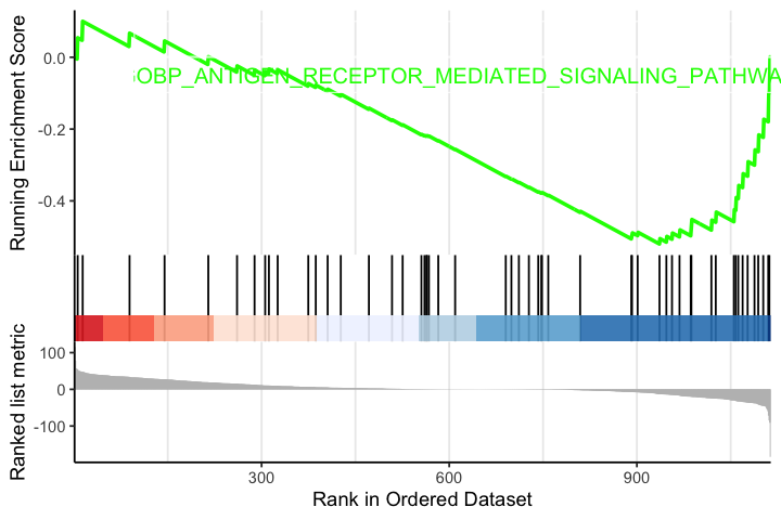
原始的图不够漂亮,优化可以参考阿汤哥的paper
这个图的代码不错,不知道他们paper里有没有分享。
2019 - Single-cell RNA-seq analysis reveals the progression of human osteoarthritis

 浙公网安备 33010602011771号