Pytorch之Spatial-Shift-Operation的5种实现策略
Pytorch之Spatial-Shift-Operation的5种实现策略
本文已授权极市平台, 并首发于极市平台公众号. 未经允许不得二次转载.
原始文档(可能会进一步更新): https://www.yuque.com/lart/ugkv9f/nnor5p
前言
之前看了一些使用空间偏移操作来替代区域卷积运算的论文:
- 粗看: https://www.yuque.com/lart/architecture/conv#uKY5N
- (CVPR 2018) [Grouped Shift] Shift: A Zero FLOP, Zero Parameter Alternative to Spatial Convolutions:
- (ICCV 2019) 4-Connected Shift Residual Networks
- (NIPS 2018) [Active Shift] Constructing Fast Network through Deconstruction of Convolution
- (CVPR 2019) [Sparse Shift] All You Need Is a Few Shifts: Designing Efficient Convolutional Neural Networks for Image Classification
- 细看:
- Vision MLP之Hire-MLP Vision MLP via Hierarchical Rearrangement
- Hire-MLP: Vision MLP via Hierarchical Rearrangement:https://www.yuque.com/lart/papers/lbhadn
- Visoin MLP之CycleMLP A MLP-like Architecture for Dense Prediction
- CycleMLP: A MLP-like Architecture for Dense Prediction:https://www.yuque.com/lart/papers/om3xb6
- Vision MLP之S2-MLP V1&V2 Spatial-Shift MLP Architecture for Vision
- S2-MLP: Spatial-Shift MLP Architecture for Vision:https://www.yuque.com/lart/papers/dgdu2b
- S2-MLPv2: Improved Spatial-Shift MLP Architecture for Vision:https://www.yuque.com/lart/papers/dgdu2b
- Vision MLP之Hire-MLP Vision MLP via Hierarchical Rearrangement
看完这些论文后, 通过参考他们提供的核心代码(主要是后面那些MLP方法), 让我对于实现空间偏移有了一些想法.
通过整合现有的知识, 我归纳总结了五种实现策略.
由于我个人使用pytorch, 所以这里的展示也可能会用到pytorch自身提供的一些有用的函数.
问题描述
在提供实现之前, 我们应该先明确目的以便于后续的实现.
这些现有的工作都可以简化为:
给定tensor \(X \in \mathbb{R}^{1 \times 8 \times 5 \times 5}\), 这里遵循pytorch默认的数据格式, 即
B, C, H, W.通过变换操作\(\mathcal{T}: x \rightarrow \tilde{x}\), 将\(X\)转换为\(\tilde{X}\).
这里tensor \(\tilde{X} \in \mathbb{R}^{1 \times 8 \times 5 \times 5}\), 为了提供合理的对比, 这里统一使用后面章节中基于"切片索引"策略的结果作为\(\tilde{X}\)的值.
import torch

xs = torch.meshgrid(torch.arange(5), torch.arange(5))
x = torch.stack(xs, dim=0)
x = x.unsqueeze(0).repeat(1, 4, 1, 1).float()
print(x)

'''
tensor([[[[0., 0., 0., 0., 0.],
          [1., 1., 1., 1., 1.],
          [2., 2., 2., 2., 2.],
          [3., 3., 3., 3., 3.],
          [4., 4., 4., 4., 4.]],

         [[0., 1., 2., 3., 4.],
          [0., 1., 2., 3., 4.],
          [0., 1., 2., 3., 4.],
          [0., 1., 2., 3., 4.],
          [0., 1., 2., 3., 4.]],

         [[0., 0., 0., 0., 0.],
          [1., 1., 1., 1., 1.],
          [2., 2., 2., 2., 2.],
          [3., 3., 3., 3., 3.],
          [4., 4., 4., 4., 4.]],

         [[0., 1., 2., 3., 4.],
          [0., 1., 2., 3., 4.],
          [0., 1., 2., 3., 4.],
          [0., 1., 2., 3., 4.],
          [0., 1., 2., 3., 4.]]]])
'''
方法1: 切片索引
这是最直接和简单的策略了. 这也是S2-MLP系列中使用的策略.
我们将其作为其他所有策略的参考对象. 后续的实现中同样会得到这个结果.
direct_shift = torch.clone(x)
direct_shift[:, 0:2, :, 1:] = torch.clone(direct_shift[:, 0:2, :, :4])
direct_shift[:, 2:4, :, :4] = torch.clone(direct_shift[:, 2:4, :, 1:])
direct_shift[:, 4:6, 1:, :] = torch.clone(direct_shift[:, 4:6, :4, :])
direct_shift[:, 6:8, :4, :] = torch.clone(direct_shift[:, 6:8, 1:, :])
print(direct_shift)

'''
tensor([[[[0., 0., 0., 0., 0.],
          [1., 1., 1., 1., 1.],
          [2., 2., 2., 2., 2.],
          [3., 3., 3., 3., 3.],
          [4., 4., 4., 4., 4.]],

         [[0., 0., 1., 2., 3.],
          [0., 0., 1., 2., 3.],
          [0., 0., 1., 2., 3.],
          [0., 0., 1., 2., 3.],
          [0., 0., 1., 2., 3.]],

         [[0., 0., 0., 0., 0.],
          [1., 1., 1., 1., 1.],
          [2., 2., 2., 2., 2.],
          [3., 3., 3., 3., 3.],
          [4., 4., 4., 4., 4.]],

         [[1., 2., 3., 4., 4.],
          [1., 2., 3., 4., 4.],
          [1., 2., 3., 4., 4.],
          [1., 2., 3., 4., 4.],
          [1., 2., 3., 4., 4.]],

         [[0., 0., 0., 0., 0.],
          [0., 0., 0., 0., 0.],
          [1., 1., 1., 1., 1.],
          [2., 2., 2., 2., 2.],
          [3., 3., 3., 3., 3.]],

         [[0., 1., 2., 3., 4.],
          [0., 1., 2., 3., 4.],
          [0., 1., 2., 3., 4.],
          [0., 1., 2., 3., 4.],
          [0., 1., 2., 3., 4.]],

         [[1., 1., 1., 1., 1.],
          [2., 2., 2., 2., 2.],
          [3., 3., 3., 3., 3.],
          [4., 4., 4., 4., 4.],
          [4., 4., 4., 4., 4.]],

         [[0., 1., 2., 3., 4.],
          [0., 1., 2., 3., 4.],
          [0., 1., 2., 3., 4.],
          [0., 1., 2., 3., 4.],
          [0., 1., 2., 3., 4.]]]])
'''
方法2: 特征图偏移—— torch.roll
pytorch提供了一个直接对特征图进行偏移的函数, 即 torch.roll . 这一操作在最近的transformer论文和mlp中有一些工作已经开始使用, 例如SwinTransformer和AS-MLP.
这里展示下AS-MLP论文中提供的伪代码:
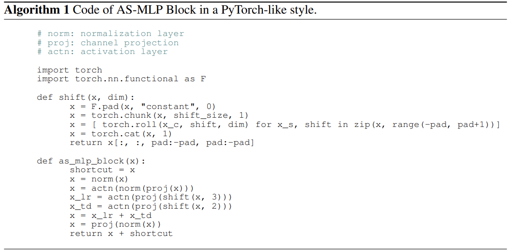
其主要作用就是将特征图沿着某个轴向进行偏移, 并支持同时沿着多个轴向偏移, 从而构造更多样的偏移方向.
为了实现与前面相同的结果, 我们需要首先对输入进行padding.
因为直接切片索引有个特点就是边界值是会重复出现的, 而若是直接roll操作, 会导致所有的值整体移动.
所以为了实现类似的效果, 先对四周各padding一个网格的数据.
注意这里选择使用重复模式(replicate)以实现最终的边界重复值的效果.
import torch.nn.functional as F

pad_x = F.pad(x, pad=[1, 1, 1, 1], mode="replicate")  # 这里需要借助padding来保留边界的数据
接下来开始处理, 沿着四个方向各偏移一个单位的长度:
roll_shift = torch.cat(
    [
        torch.roll(pad_x[:, c * 2 : (c + 1) * 2, ...], shifts=(shift_h, shift_w), dims=(2, 3))
        for c, (shift_h, shift_w) in enumerate([(0, 1), (0, -1), (1, 0), (-1, 0)])
    ],
    dim=1,
)

'''
tensor([[[[0., 0., 0., 0., 0., 0., 0.],
          [0., 0., 0., 0., 0., 0., 0.],
          [1., 1., 1., 1., 1., 1., 1.],
          [2., 2., 2., 2., 2., 2., 2.],
          [3., 3., 3., 3., 3., 3., 3.],
          [4., 4., 4., 4., 4., 4., 4.],
          [4., 4., 4., 4., 4., 4., 4.]],

         [[4., 0., 0., 1., 2., 3., 4.],
          [4., 0., 0., 1., 2., 3., 4.],
          [4., 0., 0., 1., 2., 3., 4.],
          [4., 0., 0., 1., 2., 3., 4.],
          [4., 0., 0., 1., 2., 3., 4.],
          [4., 0., 0., 1., 2., 3., 4.],
          [4., 0., 0., 1., 2., 3., 4.]],

         [[0., 0., 0., 0., 0., 0., 0.],
          [0., 0., 0., 0., 0., 0., 0.],
          [1., 1., 1., 1., 1., 1., 1.],
          [2., 2., 2., 2., 2., 2., 2.],
          [3., 3., 3., 3., 3., 3., 3.],
          [4., 4., 4., 4., 4., 4., 4.],
          [4., 4., 4., 4., 4., 4., 4.]],

         [[0., 1., 2., 3., 4., 4., 0.],
          [0., 1., 2., 3., 4., 4., 0.],
          [0., 1., 2., 3., 4., 4., 0.],
          [0., 1., 2., 3., 4., 4., 0.],
          [0., 1., 2., 3., 4., 4., 0.],
          [0., 1., 2., 3., 4., 4., 0.],
          [0., 1., 2., 3., 4., 4., 0.]],

         [[4., 4., 4., 4., 4., 4., 4.],
          [0., 0., 0., 0., 0., 0., 0.],
          [0., 0., 0., 0., 0., 0., 0.],
          [1., 1., 1., 1., 1., 1., 1.],
          [2., 2., 2., 2., 2., 2., 2.],
          [3., 3., 3., 3., 3., 3., 3.],
          [4., 4., 4., 4., 4., 4., 4.]],

         [[0., 0., 1., 2., 3., 4., 4.],
          [0., 0., 1., 2., 3., 4., 4.],
          [0., 0., 1., 2., 3., 4., 4.],
          [0., 0., 1., 2., 3., 4., 4.],
          [0., 0., 1., 2., 3., 4., 4.],
          [0., 0., 1., 2., 3., 4., 4.],
          [0., 0., 1., 2., 3., 4., 4.]],

         [[0., 0., 0., 0., 0., 0., 0.],
          [1., 1., 1., 1., 1., 1., 1.],
          [2., 2., 2., 2., 2., 2., 2.],
          [3., 3., 3., 3., 3., 3., 3.],
          [4., 4., 4., 4., 4., 4., 4.],
          [4., 4., 4., 4., 4., 4., 4.],
          [0., 0., 0., 0., 0., 0., 0.]],

         [[0., 0., 1., 2., 3., 4., 4.],
          [0., 0., 1., 2., 3., 4., 4.],
          [0., 0., 1., 2., 3., 4., 4.],
          [0., 0., 1., 2., 3., 4., 4.],
          [0., 0., 1., 2., 3., 4., 4.],
          [0., 0., 1., 2., 3., 4., 4.],
          [0., 0., 1., 2., 3., 4., 4.]]]])
'''
接下来只需要剪裁一下即可:
roll_shift = roll_shift[..., 1:6, 1:6]
print(roll_shift)

'''
tensor([[[[0., 0., 0., 0., 0.],
          [1., 1., 1., 1., 1.],
          [2., 2., 2., 2., 2.],
          [3., 3., 3., 3., 3.],
          [4., 4., 4., 4., 4.]],

         [[0., 0., 1., 2., 3.],
          [0., 0., 1., 2., 3.],
          [0., 0., 1., 2., 3.],
          [0., 0., 1., 2., 3.],
          [0., 0., 1., 2., 3.]],

         [[0., 0., 0., 0., 0.],
          [1., 1., 1., 1., 1.],
          [2., 2., 2., 2., 2.],
          [3., 3., 3., 3., 3.],
          [4., 4., 4., 4., 4.]],

         [[1., 2., 3., 4., 4.],
          [1., 2., 3., 4., 4.],
          [1., 2., 3., 4., 4.],
          [1., 2., 3., 4., 4.],
          [1., 2., 3., 4., 4.]],

         [[0., 0., 0., 0., 0.],
          [0., 0., 0., 0., 0.],
          [1., 1., 1., 1., 1.],
          [2., 2., 2., 2., 2.],
          [3., 3., 3., 3., 3.]],

         [[0., 1., 2., 3., 4.],
          [0., 1., 2., 3., 4.],
          [0., 1., 2., 3., 4.],
          [0., 1., 2., 3., 4.],
          [0., 1., 2., 3., 4.]],

         [[1., 1., 1., 1., 1.],
          [2., 2., 2., 2., 2.],
          [3., 3., 3., 3., 3.],
          [4., 4., 4., 4., 4.],
          [4., 4., 4., 4., 4.]],

         [[0., 1., 2., 3., 4.],
          [0., 1., 2., 3., 4.],
          [0., 1., 2., 3., 4.],
          [0., 1., 2., 3., 4.],
          [0., 1., 2., 3., 4.]]]])
'''
方法3: 1x1 Deformable Convolution—— ops.deform_conv2d
在阅读Cycle FC的过程中, 了解到了Deformable Convolution在实现空间偏移操作上的妙用.
由于torchvision最新版已经集成了这一操作, 所以我们只需要导入函数即可:
from torchvision.ops import deform_conv2d
为了使用它实现空间偏移, 我在对Cycle FC的解读中, 对相关代码添加了一些注释信息:
要想理解这一函数的操作, 需要首先理解后面使用的deform_conv2d_tv的具体用法.
具体可见:https://pytorch.org/vision/0.10/ops.html#torchvision.ops.deform_conv2d
这里对于offset参数的要求是:
offset (Tensor[batch_size, 2 _ offset_groups _ kernel_height * kernel_width, out_height, out_width])
offsets to be applied for each position in the convolution kernel.
也就是说, 对于样本
s的输出特征图的通道c中的位置(x, y), 这个函数会从offset中取出, 形状为kernel_height*kernel_width的卷积核所对应的偏移参数, 其为offset[s, 0:2*offset_groups*kernel_height*kernel_width, x, y]. 也就是这一系列参数都是对应样本s的单个位置(x, y)的.针对不同的位置可以有不同的
offset, 也可以有相同的 (下面的实现就是后者).对于这
2*offset_groups*kernel_height*kernel_width个数, 涉及到对于输入特征通道的分组.将其分成
offset_groups组, 每份单独拥有一组对应于卷积核中心位置的相对偏移量, 共2*kernel_height*kernel_width个数.对于每个核参数, 使用两个量来描述偏移, 即h方向和w方向相对中心位置的偏移, 即对应于后面代码中的减去
kernel_height//2或者kernel_width//2.需要注意的是, 当偏移位置位于
padding后的tensor的边界之外, 则是将网格使用0补齐. 如果网格上有边界值, 则使用边界值和用0补齐的网格顶点来计算双线性插值的结果.
该策略需要我们去构造特定的相对偏移值offset来对1x1卷积核在不同通道的采样位置进行调整.
我们先构造我们需要的offset \(\Delta \in \mathbb{R}^{1 \times 2C_iK_hK_w \times 1 \times 1}\). 这里之所以将 out_height & out_width 两个维度设置为1, 是因为我们对整个空间的偏移是一致的, 所以只需要简单的重复数值即可.
offset = torch.empty(1, 2 * 8 * 1 * 1, 1, 1)
for c, (rel_offset_h, rel_offset_w) in enumerate([(0, -1), (0, -1), (0, 1), (0, 1), (-1, 0), (-1, 0), (1, 0), (1, 0)]):
    offset[0, c * 2 + 0, 0, 0] = rel_offset_h
    offset[0, c * 2 + 1, 0, 0] = rel_offset_w
offset = offset.repeat(1, 1, 7, 7).float()  # 针对空间偏移重复偏移量
在构造offset的时候, 我们要明确, 其通道中的数据都是两两一组的, 每一组包含着沿着H轴和W轴的相对偏移量 (这一相对偏移量应该是以其作用的卷积权重位置为中心 —— 这一结论我并没有验证, 只是个人的推理, 因为这样可能在源码中实现起来更加方便, 可以直接作用权重对应位置的坐标. 在不读源码的前提下理解函数的功能, 那就需要自行构造数据来验证性的理解了).
为了更好的理解offset的作用的原理, 我们可以想象对于采样位置\((h, w)\), 使用相对偏移量\((\delta_h, \delta_w)\)作用后, 采样位置变成了\((h+\delta_h, w+\delta_w)\). 即原来作用于\((h, w)\)的权重, 偏移后直接作用到了位置\((h+\delta_h, w+\delta_w)\)上.
对于我们的前面描述的沿着四个轴向各自一个单位偏移, 可以通过对\(\delta_h\)和\(\delta_w\)分别赋予\(\{-1, 0, 1\}\)中的值即可实现.
由于这里仅需要体现通道特定的空间偏移作用, 而并不需要Deformable Convolution的卷积功能, 我们需要将卷积核设置为单位矩阵, 并转换为分组卷积对应的卷积核的形式:
weight = torch.eye(8).reshape(8, 8, 1, 1).float()
# 输入8通道,输出8通道,每个输入通道只和一个对应的输出通道有映射权值1
接下来将权重和偏移送入导入的函数中.
由于该函数对于偏移超出边界的位置是使用0补齐的网格计算的, 所以为了实现前面边界上的重复值的效果, 这里同样需要使用重复模式下的padding后的输入.
并对结果进行一下修剪:
deconv_shift = deform_conv2d(pad_x, offset=offset, weight=weight)
deconv_shift = deconv_shift[..., 1:6, 1:6]
print(deconv_shift)

'''
tensor([[[[0., 0., 0., 0., 0.],
          [1., 1., 1., 1., 1.],
          [2., 2., 2., 2., 2.],
          [3., 3., 3., 3., 3.],
          [4., 4., 4., 4., 4.]],

         [[0., 0., 1., 2., 3.],
          [0., 0., 1., 2., 3.],
          [0., 0., 1., 2., 3.],
          [0., 0., 1., 2., 3.],
          [0., 0., 1., 2., 3.]],

         [[0., 0., 0., 0., 0.],
          [1., 1., 1., 1., 1.],
          [2., 2., 2., 2., 2.],
          [3., 3., 3., 3., 3.],
          [4., 4., 4., 4., 4.]],

         [[1., 2., 3., 4., 4.],
          [1., 2., 3., 4., 4.],
          [1., 2., 3., 4., 4.],
          [1., 2., 3., 4., 4.],
          [1., 2., 3., 4., 4.]],

         [[0., 0., 0., 0., 0.],
          [0., 0., 0., 0., 0.],
          [1., 1., 1., 1., 1.],
          [2., 2., 2., 2., 2.],
          [3., 3., 3., 3., 3.]],

         [[0., 1., 2., 3., 4.],
          [0., 1., 2., 3., 4.],
          [0., 1., 2., 3., 4.],
          [0., 1., 2., 3., 4.],
          [0., 1., 2., 3., 4.]],

         [[1., 1., 1., 1., 1.],
          [2., 2., 2., 2., 2.],
          [3., 3., 3., 3., 3.],
          [4., 4., 4., 4., 4.],
          [4., 4., 4., 4., 4.]],

         [[0., 1., 2., 3., 4.],
          [0., 1., 2., 3., 4.],
          [0., 1., 2., 3., 4.],
          [0., 1., 2., 3., 4.],
          [0., 1., 2., 3., 4.]]]])
'''
方法4: 3x3 Depthwise Convolution—— F.conv2d
在S2MLP中提到了空间偏移操作可以通过使用特殊构造的3x3 Depthwise Convolution来实现.
由于基于3x3卷积操作, 所以为了实现边界值的重复效果仍然需要对输入进行重复padding.
首先构造对应四个方向的卷积核:
k1 = torch.FloatTensor([[0, 0, 0], [1, 0, 0], [0, 0, 0]]).reshape(1, 1, 3, 3)
k2 = torch.FloatTensor([[0, 0, 0], [0, 0, 1], [0, 0, 0]]).reshape(1, 1, 3, 3)
k3 = torch.FloatTensor([[0, 1, 0], [0, 0, 0], [0, 0, 0]]).reshape(1, 1, 3, 3)
k4 = torch.FloatTensor([[0, 0, 0], [0, 0, 0], [0, 1, 0]]).reshape(1, 1, 3, 3)
weight = torch.cat([k1, k1, k2, k2, k3, k3, k4, k4], dim=0)  # 每个输出通道对应一个输入通道
接下来将卷积核和数据送入 F.conv2d 中计算即可, 输入在四边各padding了1个单位, 所以输出形状不变:
conv_shift = F.conv2d(pad_x, weight=weight, groups=8)
print(conv_shift)

'''
tensor([[[[0., 0., 0., 0., 0.],
          [1., 1., 1., 1., 1.],
          [2., 2., 2., 2., 2.],
          [3., 3., 3., 3., 3.],
          [4., 4., 4., 4., 4.]],

         [[0., 0., 1., 2., 3.],
          [0., 0., 1., 2., 3.],
          [0., 0., 1., 2., 3.],
          [0., 0., 1., 2., 3.],
          [0., 0., 1., 2., 3.]],

         [[0., 0., 0., 0., 0.],
          [1., 1., 1., 1., 1.],
          [2., 2., 2., 2., 2.],
          [3., 3., 3., 3., 3.],
          [4., 4., 4., 4., 4.]],

         [[1., 2., 3., 4., 4.],
          [1., 2., 3., 4., 4.],
          [1., 2., 3., 4., 4.],
          [1., 2., 3., 4., 4.],
          [1., 2., 3., 4., 4.]],

         [[0., 0., 0., 0., 0.],
          [0., 0., 0., 0., 0.],
          [1., 1., 1., 1., 1.],
          [2., 2., 2., 2., 2.],
          [3., 3., 3., 3., 3.]],

         [[0., 1., 2., 3., 4.],
          [0., 1., 2., 3., 4.],
          [0., 1., 2., 3., 4.],
          [0., 1., 2., 3., 4.],
          [0., 1., 2., 3., 4.]],

         [[1., 1., 1., 1., 1.],
          [2., 2., 2., 2., 2.],
          [3., 3., 3., 3., 3.],
          [4., 4., 4., 4., 4.],
          [4., 4., 4., 4., 4.]],

         [[0., 1., 2., 3., 4.],
          [0., 1., 2., 3., 4.],
          [0., 1., 2., 3., 4.],
          [0., 1., 2., 3., 4.],
          [0., 1., 2., 3., 4.]]]])
'''
方法5: 网格采样—— F.grid_sample
最后这里提到的基于 F.grid_sample , 该操作是pytorch提供的用于构建STN的一个函数, 但是其在光流预测任务以及最近的一些分割任务中开始出现:
- AlignSeg: Feature-Aligned Segmentation Networks
- Semantic Flow for Fast and Accurate Scene Parsing
针对4Dtensor, 其主要作用就是根据给定的网格采样图grid\(\Gamma = \mathbb{R}^{B \times H_o \times W_o \times 2}\)来对数据点\((\gamma_h, \gamma_w)\)进行采样以放置到输出的位置\((h, w)\)中.
要注意的是, 该函数对限制了采样图grid的取值范围是对输入的尺寸归一化后的结果, 并且\(\Gamma\)的最后一维度分别是在索引W轴、H轴. 即对于输入tensor的布局 B, C, H, W 的四个维度从后往前索引. 实际上, 这一规则在pytorch的其他函数的设计中广泛遵循. 例如pytorch中的pad函数的规则也是一样的.
首先根据需求构造基于输入数据的原始坐标数组 (左上角为\((h_{coord}[0, 0], w_{coord}[0, 0])\), 右上角为\((h_{coord}[0, 5], w_{coord}[0, 5])\)):
h_coord, w_coord = torch.meshgrid(torch.arange(5), torch.arange(5))
print(h_coord)
print(w_coord)
h_coord = h_coord.reshape(1, 5, 5, 1)
w_coord = w_coord.reshape(1, 5, 5, 1)

'''
tensor([[0, 0, 0, 0, 0],
        [1, 1, 1, 1, 1],
        [2, 2, 2, 2, 2],
        [3, 3, 3, 3, 3],
        [4, 4, 4, 4, 4]])
tensor([[0, 1, 2, 3, 4],
        [0, 1, 2, 3, 4],
        [0, 1, 2, 3, 4],
        [0, 1, 2, 3, 4],
        [0, 1, 2, 3, 4]])
'''
针对每一个输出\(\tilde{x}\), 计算对应的输入\(x\)的的坐标 (即采样位置):
            torch.cat(
                [  # 请注意这里的堆叠顺序,先放靠后的轴的坐标
                    2 * torch.clamp(w_coord + w, 0, 4) / (5 - 1) - 1,
                    2 * torch.clamp(h_coord + h, 0, 4) / (5 - 1) - 1,
                ],
                dim=-1,
            )
这里的参数\(w\&h\)表示基于原始坐标系的偏移量.
由于这里直接使用clamp限制了采样区间, 靠近边界的部分会重复使用, 所以后续直接使用原始的输入即可.
将新坐标送入函数的时候, 需要将其转换为\([-1, 1]\)范围内的值, 即针对输入的形状W和H进行归一化计算.
        F.grid_sample(
            x,
            torch.cat(
                [
                    2 * torch.clamp(w_coord + w, 0, 4) / (5 - 1) - 1,
                    2 * torch.clamp(h_coord + h, 0, 4) / (5 - 1) - 1,
                ],
                dim=-1,
            ),
            mode="bilinear",
            align_corners=True,
        )
要注意, 这里使用的是 align_corners=True , 关于pytorch中该参数的介绍可以查看https://www.yuque.com/lart/idh721/ugwn46.
True :
False :
所以可以看到, 这里前者更符合我们的需求, 因为这里提到的涉及双线性插值的算法(例如前面的Deformable Convolution)的实现都是将像素放到网格顶点上的 (按照这一思路理解比较符合实验现象, 我就姑且这样描述).
grid_sampled_shift = torch.cat(
    [
        F.grid_sample(
            x,
            torch.cat(
                [
                    2 * torch.clamp(w_coord + w, 0, 4) / (5 - 1) - 1,
                    2 * torch.clamp(h_coord + h, 0, 4) / (5 - 1) - 1,
                ],
                dim=-1,
            ),
            mode="bilinear",
            align_corners=True,
        )
        for x, (h, w) in zip(x.chunk(4, dim=1), [(0, -1), (0, 1), (-1, 0), (1, 0)])
    ],
    dim=1,
)
print(grid_sampled_shift)

'''
tensor([[[[0., 0., 0., 0., 0.],
          [1., 1., 1., 1., 1.],
          [2., 2., 2., 2., 2.],
          [3., 3., 3., 3., 3.],
          [4., 4., 4., 4., 4.]],

         [[0., 0., 1., 2., 3.],
          [0., 0., 1., 2., 3.],
          [0., 0., 1., 2., 3.],
          [0., 0., 1., 2., 3.],
          [0., 0., 1., 2., 3.]],

         [[0., 0., 0., 0., 0.],
          [1., 1., 1., 1., 1.],
          [2., 2., 2., 2., 2.],
          [3., 3., 3., 3., 3.],
          [4., 4., 4., 4., 4.]],

         [[1., 2., 3., 4., 4.],
          [1., 2., 3., 4., 4.],
          [1., 2., 3., 4., 4.],
          [1., 2., 3., 4., 4.],
          [1., 2., 3., 4., 4.]],

         [[0., 0., 0., 0., 0.],
          [0., 0., 0., 0., 0.],
          [1., 1., 1., 1., 1.],
          [2., 2., 2., 2., 2.],
          [3., 3., 3., 3., 3.]],

         [[0., 1., 2., 3., 4.],
          [0., 1., 2., 3., 4.],
          [0., 1., 2., 3., 4.],
          [0., 1., 2., 3., 4.],
          [0., 1., 2., 3., 4.]],

         [[1., 1., 1., 1., 1.],
          [2., 2., 2., 2., 2.],
          [3., 3., 3., 3., 3.],
          [4., 4., 4., 4., 4.],
          [4., 4., 4., 4., 4.]],

         [[0., 1., 2., 3., 4.],
          [0., 1., 2., 3., 4.],
          [0., 1., 2., 3., 4.],
          [0., 1., 2., 3., 4.],
          [0., 1., 2., 3., 4.]]]])
'''
另外的一些思考
关于 F.grid_sample 的误差问题
由于 F.grid_sample 涉及到归一化操作, 自然而然存在精度损失.
所以实际上如果想要实现精确控制的话, 不太建议使用这个方法.
如果位置恰好在但单元格角点上, 倒是可以使用最近邻插值的模式来获得一个更加整齐的结果.
下面是一个例子:
h_coord, w_coord = torch.meshgrid(torch.arange(7), torch.arange(7))
h_coord = h_coord.reshape(1, 7, 7, 1)
w_coord = w_coord.reshape(1, 7, 7, 1)
grid = torch.cat(
    [
        2 * torch.clamp(w_coord, 0, 6) / (7 - 1) - 1,
        2 * torch.clamp(h_coord, 0, 6) / (7 - 1) - 1,
    ],
    dim=-1,
)
print(grid)
print(pad_x[:, :2])

print("mode=bilinear\n", F.grid_sample(pad_x[:, :2], grid, mode="bilinear", align_corners=True))
print("mode=nearest\n", F.grid_sample(pad_x[:, :2], grid, mode="nearest", align_corners=True))

'''
tensor([[[[-1.0000, -1.0000],
          [-0.6667, -1.0000],
          [-0.3333, -1.0000],
          [ 0.0000, -1.0000],
          [ 0.3333, -1.0000],
          [ 0.6667, -1.0000],
          [ 1.0000, -1.0000]],

         [[-1.0000, -0.6667],
          [-0.6667, -0.6667],
          [-0.3333, -0.6667],
          [ 0.0000, -0.6667],
          [ 0.3333, -0.6667],
          [ 0.6667, -0.6667],
          [ 1.0000, -0.6667]],

         [[-1.0000, -0.3333],
          [-0.6667, -0.3333],
          [-0.3333, -0.3333],
          [ 0.0000, -0.3333],
          [ 0.3333, -0.3333],
          [ 0.6667, -0.3333],
          [ 1.0000, -0.3333]],

         [[-1.0000,  0.0000],
          [-0.6667,  0.0000],
          [-0.3333,  0.0000],
          [ 0.0000,  0.0000],
          [ 0.3333,  0.0000],
          [ 0.6667,  0.0000],
          [ 1.0000,  0.0000]],

         [[-1.0000,  0.3333],
          [-0.6667,  0.3333],
          [-0.3333,  0.3333],
          [ 0.0000,  0.3333],
          [ 0.3333,  0.3333],
          [ 0.6667,  0.3333],
          [ 1.0000,  0.3333]],

         [[-1.0000,  0.6667],
          [-0.6667,  0.6667],
          [-0.3333,  0.6667],
          [ 0.0000,  0.6667],
          [ 0.3333,  0.6667],
          [ 0.6667,  0.6667],
          [ 1.0000,  0.6667]],

         [[-1.0000,  1.0000],
          [-0.6667,  1.0000],
          [-0.3333,  1.0000],
          [ 0.0000,  1.0000],
          [ 0.3333,  1.0000],
          [ 0.6667,  1.0000],
          [ 1.0000,  1.0000]]]])
tensor([[[[0., 0., 0., 0., 0., 0., 0.],
          [0., 0., 0., 0., 0., 0., 0.],
          [1., 1., 1., 1., 1., 1., 1.],
          [2., 2., 2., 2., 2., 2., 2.],
          [3., 3., 3., 3., 3., 3., 3.],
          [4., 4., 4., 4., 4., 4., 4.],
          [4., 4., 4., 4., 4., 4., 4.]],

         [[0., 0., 1., 2., 3., 4., 4.],
          [0., 0., 1., 2., 3., 4., 4.],
          [0., 0., 1., 2., 3., 4., 4.],
          [0., 0., 1., 2., 3., 4., 4.],
          [0., 0., 1., 2., 3., 4., 4.],
          [0., 0., 1., 2., 3., 4., 4.],
          [0., 0., 1., 2., 3., 4., 4.]]]])
mode=bilinear
 tensor([[[[0.0000e+00, 0.0000e+00, 0.0000e+00, 0.0000e+00, 0.0000e+00,
           0.0000e+00, 0.0000e+00],
          [1.1921e-07, 1.1921e-07, 1.1921e-07, 1.1921e-07, 1.1921e-07,
           1.1921e-07, 1.1921e-07],
          [1.0000e+00, 1.0000e+00, 1.0000e+00, 1.0000e+00, 1.0000e+00,
           1.0000e+00, 1.0000e+00],
          [2.0000e+00, 2.0000e+00, 2.0000e+00, 2.0000e+00, 2.0000e+00,
           2.0000e+00, 2.0000e+00],
          [3.0000e+00, 3.0000e+00, 3.0000e+00, 3.0000e+00, 3.0000e+00,
           3.0000e+00, 3.0000e+00],
          [4.0000e+00, 4.0000e+00, 4.0000e+00, 4.0000e+00, 4.0000e+00,
           4.0000e+00, 4.0000e+00],
          [4.0000e+00, 4.0000e+00, 4.0000e+00, 4.0000e+00, 4.0000e+00,
           4.0000e+00, 4.0000e+00]],

         [[0.0000e+00, 1.1921e-07, 1.0000e+00, 2.0000e+00, 3.0000e+00,
           4.0000e+00, 4.0000e+00],
          [0.0000e+00, 1.1921e-07, 1.0000e+00, 2.0000e+00, 3.0000e+00,
           4.0000e+00, 4.0000e+00],
          [0.0000e+00, 1.1921e-07, 1.0000e+00, 2.0000e+00, 3.0000e+00,
           4.0000e+00, 4.0000e+00],
          [0.0000e+00, 1.1921e-07, 1.0000e+00, 2.0000e+00, 3.0000e+00,
           4.0000e+00, 4.0000e+00],
          [0.0000e+00, 1.1921e-07, 1.0000e+00, 2.0000e+00, 3.0000e+00,
           4.0000e+00, 4.0000e+00],
          [0.0000e+00, 1.1921e-07, 1.0000e+00, 2.0000e+00, 3.0000e+00,
           4.0000e+00, 4.0000e+00],
          [0.0000e+00, 1.1921e-07, 1.0000e+00, 2.0000e+00, 3.0000e+00,
           4.0000e+00, 4.0000e+00]]]])
mode=nearest
 tensor([[[[0., 0., 0., 0., 0., 0., 0.],
          [0., 0., 0., 0., 0., 0., 0.],
          [1., 1., 1., 1., 1., 1., 1.],
          [2., 2., 2., 2., 2., 2., 2.],
          [3., 3., 3., 3., 3., 3., 3.],
          [4., 4., 4., 4., 4., 4., 4.],
          [4., 4., 4., 4., 4., 4., 4.]],

         [[0., 0., 1., 2., 3., 4., 4.],
          [0., 0., 1., 2., 3., 4., 4.],
          [0., 0., 1., 2., 3., 4., 4.],
          [0., 0., 1., 2., 3., 4., 4.],
          [0., 0., 1., 2., 3., 4., 4.],
          [0., 0., 1., 2., 3., 4., 4.],
          [0., 0., 1., 2., 3., 4., 4.]]]])
'''
F.grid_sample 与Deformable Convolution的关系
虽然二者都实现了对于输入与输出位置映射关系的调整, 但是二者调整的方式有着明显的差别.
- 参考坐标系不同
- 前者的坐标系是基于整体输入的一个归一化坐标系, 原点为输入的HW平面的中心位置, H轴和W轴分别以向下和向右为正向. 而在坐标系WOH中, 输入数据的左上角为\((-1, -1)\), 右上角为\((1, -1)\).
- 后者的坐标系是相对于权重初始作用位置的相对坐标系. 但是实际上, 这里其实理解为沿着H轴和W轴的_相对偏移量_更为合适. 例如, 将权重作用位置向左偏移一个单位, 实际上让其对应的偏移参数组\((\delta_h, \delta_w)\)取值为\((0, -1)\)即可, 即将作用位置相对于原始作用位置的\(w\)坐标加上个\(-1\).
- 作用效果不同
- 前者直接对整体输入进行坐标调整, 对于输入的所有通道具有相同的调整效果.
- 后者由于构建于卷积操作之上, 所以可以更加方便的处理不同通道(
offset_groups)、不同的实际上可能有重叠的局部区域(kernel_height * kernel_width). 所以实际功能更加灵活和可调整.
Shift操作的第二春
虽然在之前的工作中已经探索了多种空间shift操作的形式, 但是却并没有引起太多的关注.
- (CVPR 2018) [Grouped Shift] Shift: A Zero FLOP, Zero Parameter Alternative to Spatial Convolutions:
- (ICCV 2019) 4-Connected Shift Residual Networks
- (NIPS 2018) [Active Shift] Constructing Fast Network through Deconstruction of Convolution
- (CVPR 2019) [Sparse Shift] All You Need Is a Few Shifts: Designing Efficient Convolutional Neural Networks for Image Classification
这些工作大多专注于轻量化网络的设计, 而现在的这些基于shift的方法, 则结合了MLP这一快船, 好像又激起了一些新的水花.
当前的这些方法, 往往会采用更有效的训练设定, 这些模型之外的策略在一定程度上也极大的提升了模型的表现. 这其实也会让人疑惑, 如果直接迁移之前的那些shift操作到这里的MLP框架中, 或许性能也不会差吧?
这一想法其实也适用于传统的CNN方法, 之前的那些结构如果使用相同的训练策略, 相比现在, 到底能差多少? 这估计只能那些有卡有时间有耐心的大佬们能够一探究竟了.
实际上综合来看, 现有的这些基于空间偏移的MLP的方法, 更可以看作是 (NIPS 2018) [Active Shift] Constructing Fast Network through Deconstruction of Convolution 这篇工作的特化版本.
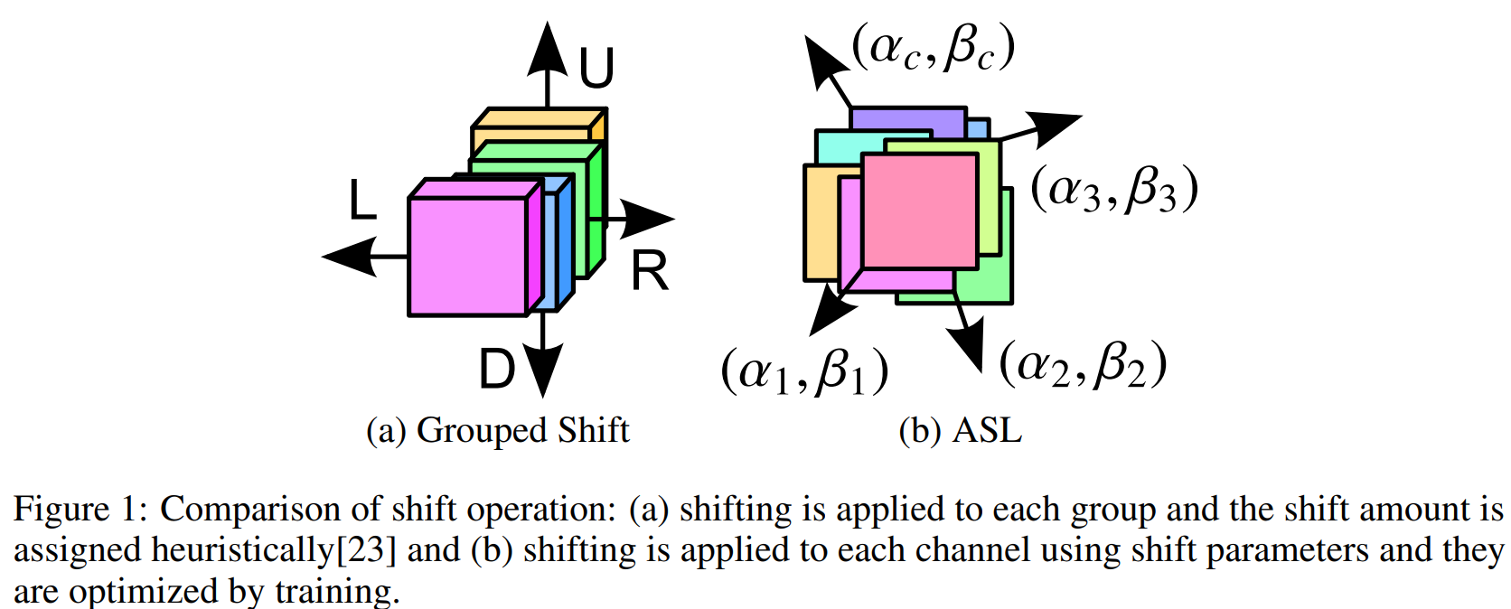
也就是将原本这篇工作中的自适应学习的偏移参数改成了固定的偏移参数.

 浙公网安备 33010602011771号