逻辑回归算法实验

【实验目的】

理解逻辑回归算法原理，掌握逻辑回归算法框架；
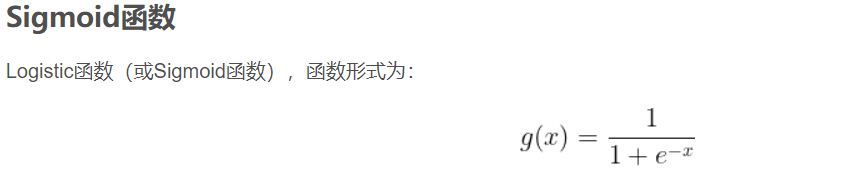
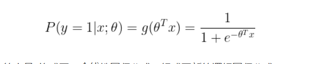
理解逻辑回归的sigmoid函数；
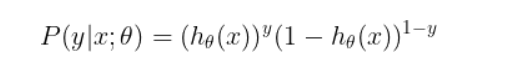
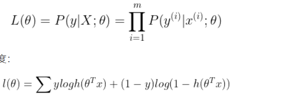
理解逻辑回归的损失函数；
针对特定应用场景及数据，能应用逻辑回归算法解决实际分类问题。

【实验内容】

1.根据给定的数据集，编写python代码完成逻辑回归算法程序，实现如下功能：

建立一个逻辑回归模型来预测一个学生是否会被大学录取。假设您是大学部门的管理员，您想根据申请人的两次考试成绩来确定他们的入学机会。您有来自以前申请人的历史数据，可以用作逻辑回归的训练集。对于每个培训示例，都有申请人的两次考试成绩和录取决定。您的任务是建立一个分类模型，根据这两门考试的分数估计申请人被录取的概率。
算法步骤与要求：

(1)读取数据；(2)绘制数据观察数据分布情况；(3)编写sigmoid函数代码；(4)编写逻辑回归代价函数代码；(5)编写梯度函数代码；(6)编写寻找最优化参数代码（可使用scipy.opt.fmin_tnc()函数）；(7)编写模型评估（预测）代码，输出预测准确率；(8)寻找决策边界，画出决策边界直线图。

2. 针对iris数据集，应用sklearn库的逻辑回归算法进行类别预测。

要求：

（1）使用seaborn库进行数据可视化；（2）将iri数据集分为训练集和测试集(两者比例为8:2)进行三分类训练和预测；（3）输出分类结果的混淆矩阵。

【实验报告要求】

对照实验内容，撰写实验过程、算法及测试结果；
代码规范化：命名规则、注释；
实验报告中需要显示并说明涉及的数学原理公式；
查阅文献，讨论逻辑回归算法的应用场景；

【实验过程及实现】

1.根据给定的数据集，编写python代码完成逻辑回归算法程序

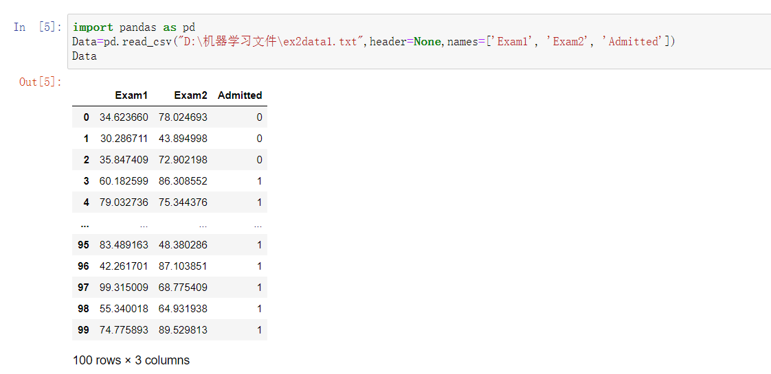
(1)导入数据

import pandas as pd
Data=pd.read_csv("D:\机器学习文件\ex2data1.txt",header=None,names=['Exam1', 'Exam2', 'Admitted'])
Data

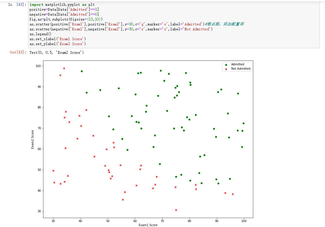
(2)绘制数据观察数据分布情况

import matplotlib.pyplot as plt
positive=Data[Data["Admitted"]==1]
negative=Data[Data["Admitted"]==0]
fig,ax=plt.subplots(figsize=(13,10))
ax.scatter(positive['Exam1'],positive['Exam2'],s=30,c='g',marker='o',label='Admitted')#散点图，添加配置项
ax.scatter(negative['Exam1'],negative['Exam2'],s=30,c='r',marker='x',label='Not Admitted')
ax.legend() 
ax.set_xlabel('Exam1 Score')
ax.set_ylabel('Exam2 Score')

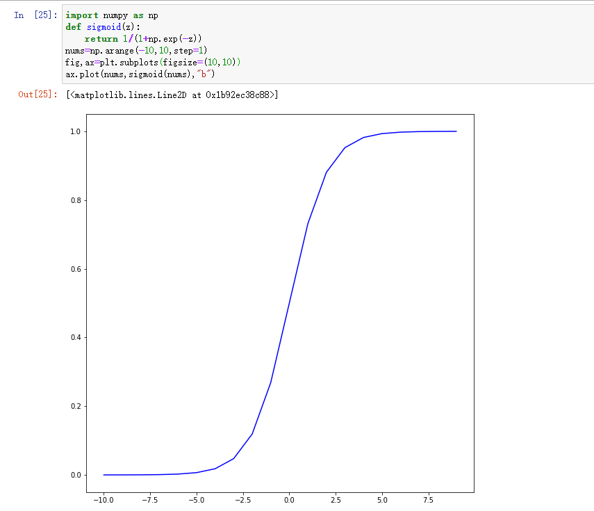
(3)编写sigmoid函数代码

import numpy as np
def sigmoid(z):
    return 1/(1+np.exp(-z))
nums=np.arange(-10,10,step=1)
fig,ax=plt.subplots(figsize=(10,10))
ax.plot(nums,sigmoid(nums),"b")

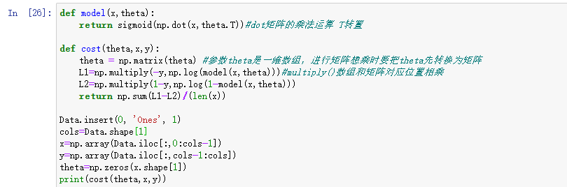
(4)编写逻辑回归代价函数代码

def model(x,theta):
    return sigmoid(np.dot(x,theta.T))#dot矩阵的乘法运算 T转置

def cost(theta,x,y):
    theta = np.matrix(theta) #参数theta是一维数组，进行矩阵想乘时要把theta先转换为矩阵
    L1=np.multiply(-y,np.log(model(x,theta)))#multiply()数组和矩阵对应位置相乘
    L2=np.multiply(1-y,np.log(1-model(x,theta)))
    return np.sum(L1-L2)/(len(x))

Data.insert(0, 'Ones', 1)
cols=Data.shape[1]
x=np.array(Data.iloc[:,0:cols-1])
y=np.array(Data.iloc[:,cols-1:cols])
theta=np.zeros(x.shape[1])
print(cost(theta,x,y))

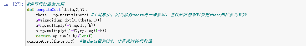
代价函数

#编写代价函数代码
def computeCost(theta,X,Y):
    theta = np.matrix(theta) #不能缺少，因为参数theta是一维数组，进行矩阵想乘时要把theta先转换为矩阵
    h=sigmoid(np.dot(X,(theta.T)))
    a=np.multiply(-Y,np.log(h))
    b=np.multiply((1-Y),np.log(1-h))
    return np.sum(a-b)/len(X)
computeCost(theta,X,Y)  #当theta值为0时，计算此时的代价值

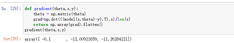
(5)编写梯度函数代码

def gradient(theta,x,y):
    theta = np.matrix(theta) 
    grad=np.dot(((model(x,theta)-y).T),x)/len(x)
    return np.array(grad).flatten()
gradient(theta,x,y)

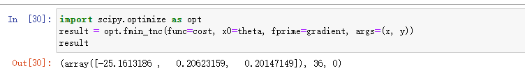
(6)寻找最优化参数

import scipy.optimize as opt
result = opt.fmin_tnc(func=cost, x0=theta, fprime=gradient, args=(x, y))
result

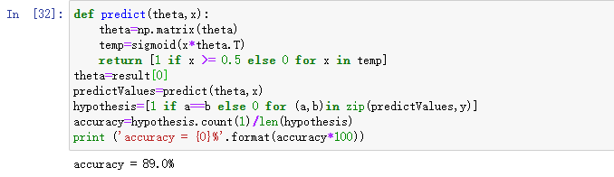
(7)编写模型评估代码，输出预测准确率

def predict(theta,x):
    theta=np.matrix(theta)
    temp=sigmoid(x*theta.T)
    return [1 if x >= 0.5 else 0 for x in temp]
theta=result[0]
predictValues=predict(theta,x)
hypothesis=[1 if a==b else 0 for (a,b)in zip(predictValues,y)]
accuracy=hypothesis.count(1)/len(hypothesis)
print ('accuracy = {0}%'.format(accuracy*100))

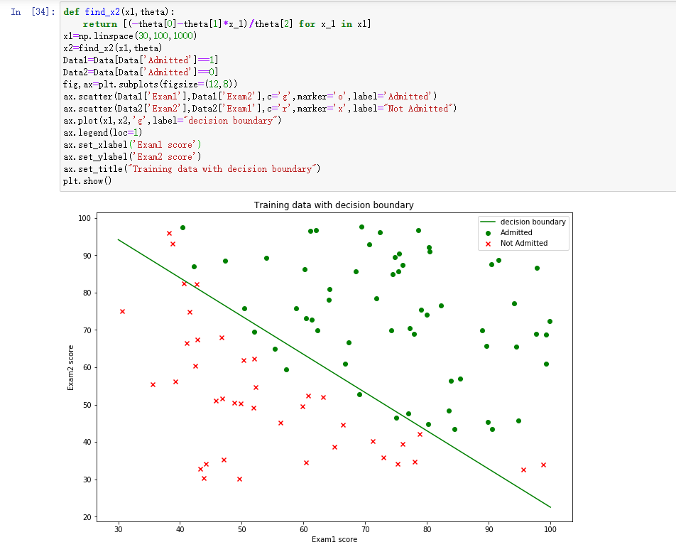
(8)寻找决策边界，画出决策边界直线图

def find_x2(x1,theta):
    return [(-theta[0]-theta[1]*x_1)/theta[2] for x_1 in x1]
x1=np.linspace(30,100,1000)
x2=find_x2(x1,theta)
Data1=Data[Data['Admitted']==1]
Data2=Data[Data['Admitted']==0]
fig,ax=plt.subplots(figsize=(12,8))
ax.scatter(Data1['Exam1'],Data1['Exam2'],c='b',marker='o',label='Admitted')
ax.scatter(Data2['Exam2'],Data2['Exam1'],c='r',marker='x',label="Not Admitted")
ax.plot(x1,x2,'g',label="decision boundary")
ax.legend(loc=1)
ax.set_xlabel('Exam1 score')
ax.set_ylabel('Exam2 score')
ax.set_title("Training data with decision boundary")
plt.show()

2. 针对iris数据集，应用sklearn库的逻辑回归算法进行类别预测。

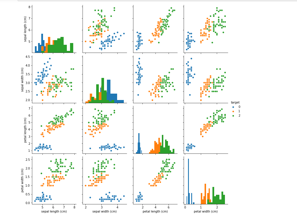
（1）使用seaborn库进行数据可视化

import seaborn as sns
from sklearn.datasets import load_iris# 我们利用 sklearn 中自带的 iris 数据作为数据载入，并利用Pandas转化为DataFrame格式
data=load_iris() #得到数据特征
iris_target=data.target #得到数据对应的标签
iris_features=pd.DataFrame(data=data.data, columns=data.feature_names) #利用Pandas转化为DataFrame格式
iris_features.describe()
iris_all=iris_features.copy()
iris_all['target']=iris_target
#利用value_counts函数查看每个类别数量
pd.Series(iris_target).value_counts()
sns.pairplot(data=iris_all,diag_kind='hist',hue= 'target') # pairplot用来进行数据分析，画两两特征图。
plt.show()

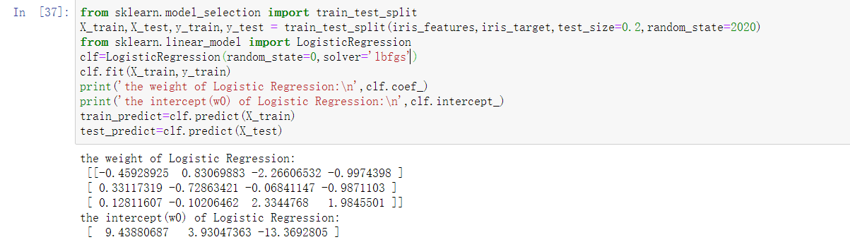
2）将iri数据集分为训练集和测试集(两者比例为8:2)进行三分类训练和预测

from sklearn.model_selection import train_test_split
X_train,X_test,y_train,y_test = train_test_split(iris_features,iris_target,test_size=0.2,random_state=2020)
from sklearn.linear_model import LogisticRegression
clf=LogisticRegression(random_state=0,solver='lbfgs')
clf.fit(X_train,y_train)
print('the weight of Logistic Regression:\n',clf.coef_)
print('the intercept(w0) of Logistic Regression:\n',clf.intercept_)
train_predict=clf.predict(X_train)
test_predict=clf.predict(X_test)

（3）输出分类结果的混淆矩阵

from sklearn import metrics
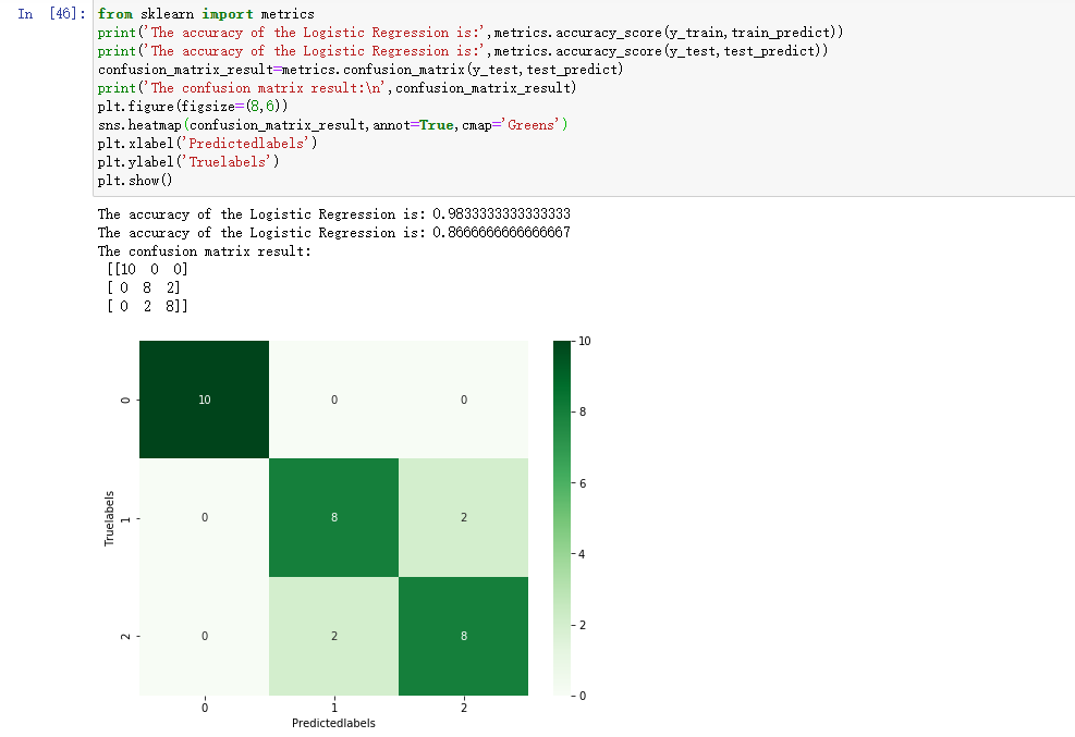
#利用accuracy（准确度）【预测正确的样本数目占总预测样本数目的比例】评估模型效果
print('The accuracy of the Logistic Regression is:',metrics.accuracy_score(y_train,train_predict))
print('The accuracy of the Logistic Regression is:',metrics.accuracy_score(y_test,test_predict))
#查看混淆矩阵(预测值和真实值的各类情况统计矩阵)
confusion_matrix_result=metrics.confusion_matrix(y_test,test_predict)
print('The confusion matrix result:\n',confusion_matrix_result)
# 利用热力图对于结果进行可视化,画混淆矩阵
plt.figure(figsize=(8,6))
sns.heatmap(confusion_matrix_result,annot=True,cmap='Greens')
plt.xlabel('Predictedlabels')
plt.ylabel('Truelabels')
plt.show()