深度学习之Tensorflow入门
声明
本文参考【中文】【吴恩达课后编程作业】Course 2 - 改善深层神经网络 - 第三周作业_何宽的博客-CSDN博客我对这篇博客加上自己的理解,力求看懂
本文所使用的资料已上传到百度网盘【点击下载】,提取码:dvrc,请在开始之前下载好所需资料,或者在本文底部copy资料代码。
到目前为止,我们一直在使用numpy来自己编写神经网络。现在我们将一步步的使用深度学习的框架来很容易的构建属于自己的神经网络。我们将学习TensorFlow这个框架:
- 初始化变量
- 建立一个会话
- 训练的算法
- 实现一个神经网络
我们知道在使用框架的时候,只需要写好前向传播就好了,这是因为在使用tensor转化为Variable后具有求导的特性,即自动记录变量的梯度相关信息
1 - 导入TensorFlow库
import numpy as np
import h5py
import matplotlib.pyplot as plt
import tensorflow as tf
import tensorflow.compat.v1 as tf #以下两行代码是因为我们的tensorflow等级太高了,我们需要给他降级
tf.disable_v2_behavior()
from tensorflow.python.framework import ops
import tf_utils
import time
np.random.seed(1)
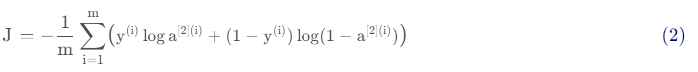
我们现在已经导入了相关的库,我们将引导你完成不同的应用,我们现在看一下下面的计算损失的公式:

y_hat = tf.constant(36,name="y_hat")            #定义y_hat为固定值36
y = tf.constant(39,name="y")                    #定义y为固定值39

loss = tf.Variable((y-y_hat)**2,name="loss" )   #为损失函数创建一个变量

init = tf.global_variables_initializer()        #运行之后的初始化(ession.run(init))
                                                #损失变量将被初始化并准备计算
with tf.Session() as session:                   #创建一个session并打印输出
    session.run(init)                           #初始化变量
    print(session.run(loss))                    #打印损失值
9
对于Tensorflow的代码实现而言,实现代码的结构如下:
-
创建Tensorflow变量(此时,尚未直接计算)
-
实现Tensorflow变量之间的操作定义
-
初始化Tensorflow变量
-
创建Session
-
运行Session,此时,之前编写操作都会在这一步运行。
因此,当我们为损失函数创建一个变量时,我们简单地将损失定义为其他数量的函数,但没有评估它的价值。 为了评估它,我们需要运行init=tf.global_variables_initializer(),初始化损失变量,在最后一行,我们最后能够评估损失的值并打印它的值。
现在让我们看一个简单的例子:
a = tf.constant(2) # 定义常量,普通的tensor
b = tf.constant(10)
c = tf.multiply(a,b)

print(c)
Tensor("Mul:0", shape=(), dtype=int32)
并没有输出具体的值,是因为我们还没有创建Session
sess = tf.Session() # 创建Session
print(sess.run(c))
20
总结一下,记得初始化变量,然后创建一个session来运行它。
接下来,我们需要了解一下占位符(placeholders)这个占位符只能是tensorflow1使用,因此我们需要降阶。占位符是一个对象,它的值只能在稍后指定,要指定占位符的值,可以使用一个feed字典(feed_dict变量)来传入,接下来,我们为x创建一个占位符,这将允许我们在稍后运行会话时传入一个数字。
x = tf.placeholder(tf.int64,name='x')
print(sess.run(2*x,feed_dict={x:3}))
6
当我们第一次定义x时,我们不必为它指定一个值。 占位符只是一个变量,我们会在运行会话时将数据分配给它。
线性函数
让我们通过计算以下等式来开始编程:Y = WX + b ,W和X是随机矩阵,b是随机向量。
我们计算WX + b ,其中W,X 和b是从随机正态分布中抽取的。 W的维度是(4,3),X 是(3,1),b 是(4,1)。 我们开始定义一个shape=(3,1)的常量X:
def linear_function():
    """
    实现一个线性功能:
        初始化W,类型为tensor的随机变量,维度为(4,3)
        初始化X,类型为tensor的随机变量,维度为(3,1)
        初始化b,类型为tensor的随机变量,维度为(4,1)
    返回:
        result - 运行了session后的结果,运行的是Y = WX + b

    """
    np.random.seed(1)
    x = tf.constant(np.random.randn(3,1),name = 'x')


    w = np.random.randn(4,3)
    b = np.random.randn(4,1)

    Y = tf.add(tf.matmul(w,x),b)
    sess = tf.Session()
    result = sess.run(Y)
    sess.close() # 使用完记得关闭

    return result
我们来测试一下:
print('result = ' + str(linear_function()))
result = [[-2.15657382]
 [ 2.95891446]
 [-1.08926781]
 [-0.84538042]]
计算sigmoid
我们已经实现了线性函数,TensorFlow提供了多种常用的神经网络的函数比如tf.softmax和 tf.sigmoid。
我们将使用占位符变量x,当运行这个session的时候,我们西药使用使用feed字典来输入z,我们将创建占位符变量x,使用tf.sigmoid来定义操作符,最后运行session,我们会用到下面的代码:
tf.placeholder(tf.float32, name = “…”)
tf.sigmoid(…)
sess.run(…, feed_dict = {x: z})
def sigmoid(z):
    """
    实现使用sigmoid函数计算z

    参数:
        z - 输入的值,标量或矢量

    返回:
        result - 用sigmoid计算z的值

    """
    x = tf.placeholder(tf.float32,name='x')
    sigmoid = tf.sigmoid(x)
    with tf.Session() as sess:
        result = sess.run(sigmoid,feed_dict = {x:z})
    return result
我们测试一下:
print('sigmoid(0) = ' + str(sigmoid(0)))
print('sigimoid(12) = ' + str(sigmoid(12)))
sigmoid(0) = 0.5
sigimoid(12) = 0.99999386
计算成本
实现成本函数,需要用到的是:
tf.nn.sigmoid_cross_entropy_with_logits(logits = ..., labels = ...)
你的代码应该输入z,计算sigmoid(得到 a),然后计算交叉熵成本J ,所有的步骤都可以通过一次调用tf.nn.sigmoid_cross_entropy_with_logits来完成。
使用独热编码(0、1编码)
很多时候在深度学习中y yy向量的维度是从0 到C − 1的,C 是指分类的类别数量,如果C = 4 ,那么对y 而言你可能需要有以下的转换方式: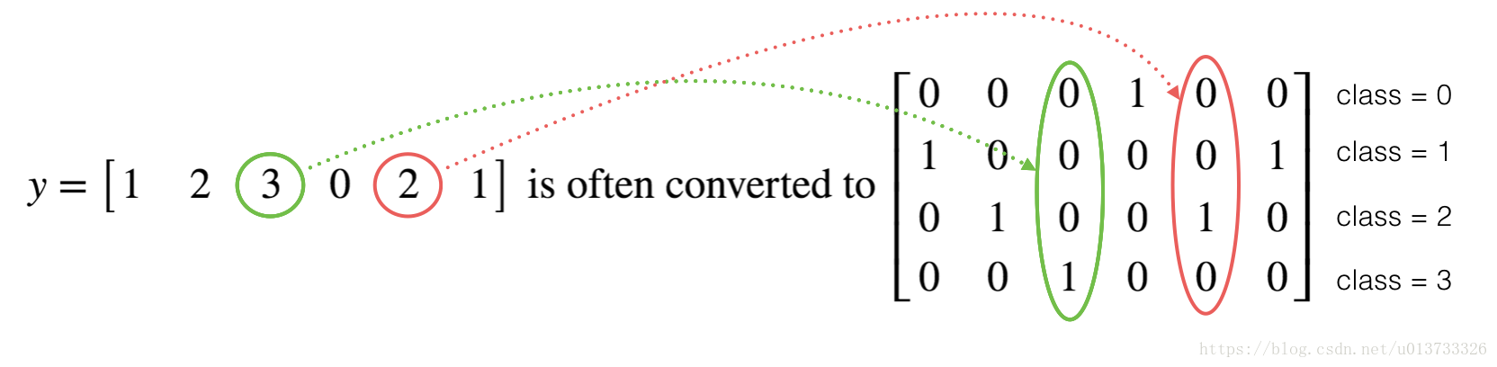
下面我们要做的是取一个标签矢量和C类总数,返回一个独热编码。
def one_hot_matrix(labels,C):
    """
    创建一个矩阵,其中第i行对应第i个类号,第j列对应第j个训练样本
    所以如果第j个样本对应着第i个标签,那么entry (i,j)将会是1

    参数:
        lables - 标签向量
        C - 分类数

    返回:
        one_hot - 独热矩阵

    """
    C = tf.constant(C,name='C')
    one_hot_matrix = tf.one_hot(indices=labels,depth = C ,axis =0)
    sess = tf.Session()
    one_hot = sess.run(one_hot_matrix)
    sess.close()
    return(str(one_hot))
测试一下:
labels = np.array([1,2,3,0,2,1])
one_hot = one_hot_matrix(labels,C = 4)
print(str(one_hot))
[[0. 0. 0. 1. 0. 0.]
 [1. 0. 0. 0. 0. 1.]
 [0. 1. 0. 0. 1. 0.]
 [0. 0. 1. 0. 0. 0.]]
初始化为0和1
现在我们将学习如何用0或者1初始化一个向量,我们要用到tf.ones()和tf.zeros(),给定这些函数一个维度值那么它们将会返回全是1或0的满足条件的向量/矩阵,我们来看看怎样实现它们:
def ones(shape):
    ones = tf.ones(shape)
    sess = tf.Session()
    ones = sess.run(ones)
    sess.close()
    return ones
测试一下:
print('ones = '+ str(ones([4,4])))
ones = [[1. 1. 1. 1.]
 [1. 1. 1. 1.]
 [1. 1. 1. 1.]
 [1. 1. 1. 1.]]
使用TensorFlow构建你的第一个神经网络
这里就是一个one_hot一个类型
首先我们需要加载数据集:
X_train_orig , Y_train_orig , X_test_orig , Y_test_orig , classes = tf_utils.load_dataset()
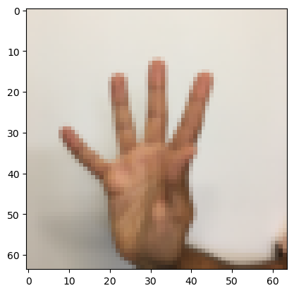
让我们看看数据集里面有什么
index = 12
plt.imshow(X_train_orig[index])
print('Y = ' + str(np.squeeze(Y_train_orig[:,index])))
Y = 5
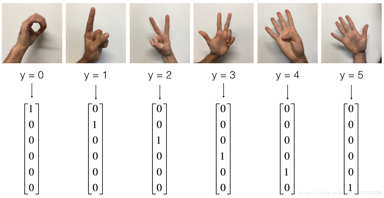
和往常一样,我们要对数据集进行扁平化,然后再除以255以归一化数据,除此之外,我们要需要把每个标签转化为独热向量,像上面的图一样。
X_train_flatten = X_train_orig.reshape(X_train_orig.shape[0],-1).T #每一列就是一个样本
X_test_flatten = X_test_orig.reshape(X_test_orig.shape[0],-1).T

#归一化数据
X_train = X_train_flatten / 255
X_test = X_test_flatten / 255

#转换为独热矩阵
Y_train = tf_utils.convert_to_one_hot(Y_train_orig,6)
Y_test = tf_utils.convert_to_one_hot(Y_test_orig,6)

print("训练集样本数 = " + str(X_train.shape[1]))
print("测试集样本数 = " + str(X_test.shape[1]))
print("X_train.shape: " + str(X_train.shape))
print("Y_train.shape: " + str(Y_train.shape))
print("X_test.shape: " + str(X_test.shape))
print("Y_test.shape: " + str(Y_test.shape))
训练集样本数 = 1080
测试集样本数 = 120
X_train.shape: (12288, 1080)
Y_train.shape: (6, 1080)
X_test.shape: (12288, 120)
Y_test.shape: (6, 120)
我们的目标是构建能够高准确度识别符号的算法。 要做到这一点,你要建立一个TensorFlow模型,这个模型几乎和你之前在猫识别中使用的numpy一样(但现在使用softmax输出)。要将您的numpy实现与tensorflow实现进行比较的话这是一个很好的机会。
目前的模型是:LINEAR -> RELU -> LINEAR -> RELU -> LINEAR -> SOFTMAX,SIGMOID输出层已经转换为SOFTMAX。当有两个以上的类时,一个SOFTMAX层将SIGMOID一般化。
我的理解是,因为在深度学习出来之前就已经有numpy了,它并不适合深度学习,而tf.Tensor为了弥补numpy的缺点,更多是为了深度学习而生
创建placeholders
我们的第一项任务是为X和Y创建占位符,这将允许我们稍后在运行会话时传递您的训练数据。
def create_placeholders(n_x,n_y):
    """
    为TensorFlow会话创建占位符
    参数:
        n_x - 一个实数,图片向量的大小(64*64*3 = 12288)
        n_y - 一个实数,分类数(从0到5,所以n_y = 6)

    返回:
        X - 一个数据输入的占位符,维度为[n_x, None],dtype = "float"
        Y - 一个对应输入的标签的占位符,维度为[n_Y,None],dtype = "float"

    提示:
        使用None,因为它让我们可以灵活处理占位符提供的样本数量。事实上,测试/训练期间的样本数量是不同的。

    """

    X = tf.placeholder(tf.float32, [n_x, None], name="X")
    Y = tf.placeholder(tf.float32, [n_y, None], name="Y")

    return X, Y
测试一下:
X, Y = create_placeholders(12288, 6)
print("X = " + str(X))
print("Y = " + str(Y))
X = Tensor("X_4:0", shape=(12288, ?), dtype=float32)
Y = Tensor("Y_1:0", shape=(6, ?), dtype=float32)
初始化参数
初始化tensorflow中的参数,我们将使用Xavier初始化权重和用零来初始化偏差,比如:
在tensorflow2中已经不支持tf.contrib了,但是有tf.glorot与之代替
W1 = tf.get_variable("W1", [25,12288], initializer=tf.glorot_uniform_initializer(seed=1))
b1 = tf.get_variable("b1", [25,1], initializer = tf.zeros_initializer())
tf.Variable() 每次都在创建新对象,对于get_variable()来说,对于已经创建的变量对象,就把那个对象返回,如果没有创建变量对象的话,就创建一个新的。
def initialize_parameters():
    """
    初始化神经网络的参数,参数的维度如下:
        W1 : [25, 12288]
        b1 : [25, 1]
        W2 : [12, 25]
        b2 : [12, 1]
        W3 : [6, 12]
        b3 : [6, 1]

    返回:
        parameters - 包含了W和b的字典


    """

    tf.set_random_seed(1) #指定随机种子

    W1 = tf.get_variable("W1",[25,12288],initializer=tf.glorot_uniform_initializer(seed=1))
    b1 = tf.get_variable("b1",[25,1],initializer=tf.zeros_initializer())
    W2 = tf.get_variable("W2", [12, 25], initializer=tf.glorot_uniform_initializer(seed=1))
    b2 = tf.get_variable("b2", [12, 1], initializer = tf.zeros_initializer())
    W3 = tf.get_variable("W3", [6, 12], initializer=tf.glorot_uniform_initializer(seed=1))
    b3 = tf.get_variable("b3", [6, 1], initializer = tf.zeros_initializer())

    parameters = {"W1": W1,
                  "b1": b1,
                  "W2": W2,
                  "b2": b2,
                  "W3": W3,
                  "b3": b3}

    return parameters
测试一下:
tf.reset_default_graph() #用于清除默认图形堆栈并重置全局默认图形。

with tf.Session() as sess:
    parameters = initialize_parameters()
    print("W1 = " + str(parameters["W1"]))
    print("b1 = " + str(parameters["b1"]))
    print("W2 = " + str(parameters["W2"]))
    print("b2 = " + str(parameters["b2"]))
W1 = <tf.Variable 'W1:0' shape=(25, 12288) dtype=float32_ref>
b1 = <tf.Variable 'b1:0' shape=(25, 1) dtype=float32_ref>
W2 = <tf.Variable 'W2:0' shape=(12, 25) dtype=float32_ref>
b2 = <tf.Variable 'b2:0' shape=(12, 1) dtype=float32_ref>
前向传播
我们要实现神经网络的前向传播,我们会拿numpy与TensorFlow实现的神经网络的代码作比较。最重要的是前向传播要在Z3处停止,因为在TensorFlow中最后的线性输出层的输出作为计算损失函数的输入,所以不需要A3.
def forward_propagation(X,parameters):
    """
    实现一个模型的前向传播,模型结构为LINEAR -> RELU -> LINEAR -> RELU -> LINEAR -> SOFTMAX

    参数:
        X - 输入数据的占位符,维度为(输入节点数量,样本数量)
        parameters - 包含了W和b的参数的字典

    返回:
        Z3 - 最后一个LINEAR节点的输出

    """

    W1 = parameters['W1']
    b1 = parameters['b1']
    W2 = parameters['W2']
    b2 = parameters['b2']
    W3 = parameters['W3']
    b3 = parameters['b3']

    Z1 = tf.add(tf.matmul(W1,X),b1)        # Z1 = np.dot(W1, X) + b1
    #Z1 = tf.matmul(W1,X) + b1             #也可以这样写
    A1 = tf.nn.relu(Z1)                    # A1 = relu(Z1)
    Z2 = tf.add(tf.matmul(W2, A1), b2)     # Z2 = np.dot(W2, a1) + b2
    A2 = tf.nn.relu(Z2)                    # A2 = relu(Z2)
    Z3 = tf.add(tf.matmul(W3, A2), b3)     # Z3 = np.dot(W3,Z2) + b3


    return Z3
测试一下:
tf.reset_default_graph() #用于清除默认图形堆栈并重置全局默认图形。
with tf.Session() as sess:
    X,Y = create_placeholders(12288,6)
    parameters = initialize_parameters()
    Z3 = forward_propagation(X,parameters)
    print("Z3 = " + str(Z3))
Z3 = Tensor("Add_2:0", shape=(6, ?), dtype=float32)
计算成本
def compute_cost(Z3,Y):
    """
    计算成本

    参数:
        Z3 - 前向传播的结果
        Y - 标签,一个占位符,和Z3的维度相同

    返回:
        cost - 成本值


    """
    logits = tf.transpose(Z3) #转置
    labels = tf.transpose(Y)  #转置

    cost = tf.reduce_mean(tf.nn.softmax_cross_entropy_with_logits(logits=logits,labels=labels))


    return cost
测试一下:
tf.reset_default_graph()

with tf.Session() as sess:
    X,Y = create_placeholders(12288,6)
    parameters = initialize_parameters()
    Z3 = forward_propagation(X,parameters)
    cost = compute_cost(Z3,Y)
    print("cost = " + str(cost))
cost = Tensor("Mean:0", shape=(), dtype=float32)
构建模型
博主自己在里面想加一下L2正则化
l2_loss = tf.get_collection(tf.GraphKeys.REGULARIZATION_LOSSES)
    loss = tf.add_n([cost] + l2_loss, name="loss")
def model(X_train,Y_train,X_test,Y_test,
        learning_rate=0.0001,num_epochs=1500,minibatch_size=32,
        print_cost=True,is_plot=True):
    """
    实现一个三层的TensorFlow神经网络:LINEAR->RELU->LINEAR->RELU->LINEAR->SOFTMAX

    参数:
        X_train - 训练集,维度为(输入大小(输入节点数量) = 12288, 样本数量 = 1080)
        Y_train - 训练集分类数量,维度为(输出大小(输出节点数量) = 6, 样本数量 = 1080)
        X_test - 测试集,维度为(输入大小(输入节点数量) = 12288, 样本数量 = 120)
        Y_test - 测试集分类数量,维度为(输出大小(输出节点数量) = 6, 样本数量 = 120)
        learning_rate - 学习速率
        num_epochs - 整个训练集的遍历次数
        mini_batch_size - 每个小批量数据集的大小
        print_cost - 是否打印成本,每100代打印一次
        is_plot - 是否绘制曲线图

    返回:
        parameters - 学习后的参数

    """

    ops.reset_default_graph()                #能够重新运行模型而不覆盖tf变量
    tf.set_random_seed(1)
    seed = 3
    (n_x , m)  = X_train.shape               #获取输入节点数量和样本数
    n_y = Y_train.shape[0]                   #获取输出节点数量
    costs = []                               #成本集

    #给X和Y创建placeholder
    X,Y = create_placeholders(n_x,n_y)

    #初始化参数
    parameters = initialize_parameters()

    #前向传播
    Z3 = forward_propagation(X,parameters)

    #计算成本
    cost = compute_cost(Z3,Y)
    l2_loss = tf.get_collection(tf.GraphKeys.REGULARIZATION_LOSSES)
    loss = tf.add_n([cost] + l2_loss, name="loss")


    #反向传播,使用Adam优化
    optimizer = tf.train.AdamOptimizer(learning_rate=learning_rate).minimize(cost)

    #初始化所有的变量
    init = tf.global_variables_initializer()

    #开始会话并计算
    with tf.Session() as sess:
        #初始化
        sess.run(init)

        #正常训练的循环
        for epoch in range(num_epochs):

            epoch_cost = 0  #每代的成本
            num_minibatches = int(m / minibatch_size)    #minibatch的总数量
            seed = seed + 1
            minibatches = tf_utils.random_mini_batches(X_train,Y_train,minibatch_size,seed)

            for minibatch in minibatches:

                #选择一个minibatch
                (minibatch_X,minibatch_Y) = minibatch

                #数据已经准备好了,开始运行session
                _ , minibatch_cost = sess.run([optimizer,cost],feed_dict={X:minibatch_X,Y:minibatch_Y})

                #计算这个minibatch在这一代中所占的误差
                epoch_cost = epoch_cost + minibatch_cost / num_minibatches

            #记录并打印成本
            ## 记录成本
            if epoch % 5 == 0:
                costs.append(epoch_cost)
                #是否打印:
                if print_cost and epoch % 100 == 0:
                        print("epoch = " + str(epoch) + "    epoch_cost = " + str(epoch_cost))

        #是否绘制图谱
        if is_plot:
            plt.plot(np.squeeze(costs))
            plt.ylabel('cost')
            plt.xlabel('iterations (per tens)')
            plt.title("Learning rate =" + str(learning_rate))
            plt.show()

        #保存学习后的参数
        parameters = sess.run(parameters)
        print("参数已经保存到session。")

        #计算当前的预测结果
        correct_prediction = tf.equal(tf.argmax(Z3),tf.argmax(Y))

        #计算准确率
        accuracy = tf.reduce_mean(tf.cast(correct_prediction,"float"))

        print("训练集的准确率:", accuracy.eval({X: X_train, Y: Y_train}))
        print("测试集的准确率:", accuracy.eval({X: X_test, Y: Y_test}))

        return parameters
我们来正式运行一下模型,没有显卡是真的很慢
#开始时间
start_time = time.perf_counter()
#开始训练
parameters = model(X_train, Y_train, X_test, Y_test)
#结束时间
end_time = time.perf_counter()
#计算时差
print("CPU的执行时间 = " + str(end_time - start_time) + " 秒" )
epoch = 0    epoch_cost = 1.8557019233703616
epoch = 100    epoch_cost = 1.0172552628950642
epoch = 200    epoch_cost = 0.733183786724553
epoch = 300    epoch_cost = 0.5730706182393162
epoch = 400    epoch_cost = 0.46869878651517827
epoch = 500    epoch_cost = 0.3812084595362345
epoch = 600    epoch_cost = 0.31382483198787225
epoch = 700    epoch_cost = 0.25364145591403503
epoch = 800    epoch_cost = 0.20389534262093628
epoch = 900    epoch_cost = 0.16644860126755456
epoch = 1000    epoch_cost = 0.1466958195422635
epoch = 1100    epoch_cost = 0.10727535018866712
epoch = 1200    epoch_cost = 0.08655262428025405
epoch = 1300    epoch_cost = 0.05933702635494144
epoch = 1400    epoch_cost = 0.05227517494649599
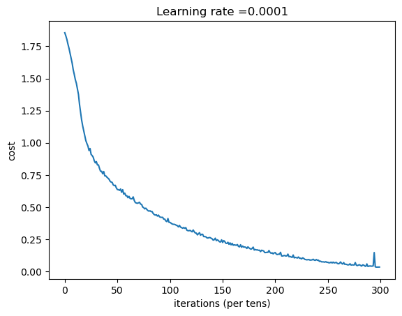
参数已经保存到session。
训练集的准确率: 0.9990741
测试集的准确率: 0.725
CPU的执行时间 = 1832.5628375000001 秒
现在,我们的算法已经可以识别0-5的手势符号了,准确率在72.5%。
我们的模型看起来足够大了,可以适应训练集,但是考虑到训练与测试的差异,你也完全可以尝试添加L2或者dropout来减少过拟合。将session视为一组代码来训练模型,在每个minibatch上运行会话时,都会训练我们的参数,总的来说,你已经运行了很多次(1500代),直到你获得训练有素的参数。
好了。让我们拍几张照片来测试一下吧!
我在做的时候在调库的时候他总是报错,就是因为tensorflow1和tensorflow2不兼容,然后经过一系列的思想斗争,最终将所使用的库拿到这里运行一下,发现不报错了
以下是我们要使用的包
def predict(X, parameters):

    W1 = tf.convert_to_tensor(parameters["W1"])
    b1 = tf.convert_to_tensor(parameters["b1"])
    W2 = tf.convert_to_tensor(parameters["W2"])
    b2 = tf.convert_to_tensor(parameters["b2"])
    W3 = tf.convert_to_tensor(parameters["W3"])
    b3 = tf.convert_to_tensor(parameters["b3"])

    params = {"W1": W1,
              "b1": b1,
              "W2": W2,
              "b2": b2,
              "W3": W3,
              "b3": b3}

    x = tf.placeholder("float", [12288, 1])

    z3 = forward_propagation_for_predict(x, params)
    p = tf.argmax(z3)

    sess = tf.Session()
    prediction = sess.run(p, feed_dict = {x: X})

    return prediction
还有这个
def forward_propagation_for_predict(X, parameters):
    """
    Implements the forward propagation for the model: LINEAR -> RELU -> LINEAR -> RELU -> LINEAR -> SOFTMAX

    Arguments:
    X -- input dataset placeholder, of shape (input size, number of examples)
    parameters -- python dictionary containing your parameters "W1", "b1", "W2", "b2", "W3", "b3"
                  the shapes are given in initialize_parameters
    Returns:
    Z3 -- the output of the last LINEAR unit
    """

    # Retrieve the parameters from the dictionary "parameters"
    W1 = parameters['W1']
    b1 = parameters['b1']
    W2 = parameters['W2']
    b2 = parameters['b2']
    W3 = parameters['W3']
    b3 = parameters['b3']
                                                           # Numpy Equivalents:
    Z1 = tf.add(tf.matmul(W1, X), b1)                      # Z1 = np.dot(W1, X) + b1
    A1 = tf.nn.relu(Z1)                                    # A1 = relu(Z1)
    Z2 = tf.add(tf.matmul(W2, A1), b2)                     # Z2 = np.dot(W2, a1) + b2
    A2 = tf.nn.relu(Z2)                                    # A2 = relu(Z2)
    Z3 = tf.add(tf.matmul(W3, A2), b3)                     # Z3 = np.dot(W3,Z2) + b3

    return Z3
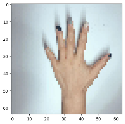
博主自己拍了6张图片,然后裁剪成1:1的样式(其实原本就是正方形的就是1:1),再通过格式工厂把很大的图片缩放成64x64的图片,同时把jpg转化为png,因为mpimg只能读取png的图片。
import matplotlib.pyplot as plt # plt 用于显示图片
import matplotlib.image as mpimg # mpimg 用于读取图片
import numpy as np

#这是我女朋友拍的图片
my_image1 = "5.png"                                            #定义图片名称
fileName1 = "C:/Users/TJRA/Desktop/" + my_image1                      #图片地址
image1 = mpimg.imread(fileName1)                               #读取图片
plt.imshow(image1)                                             #显示图片
my_image1 = image1.reshape(1,64 * 64 * 3).T                    #重构图片
my_image_prediction = predict(my_image1, parameters)  #开始预测
print("预测结果: y = " + str(np.squeeze(my_image_prediction)))
预测结果: y = 2
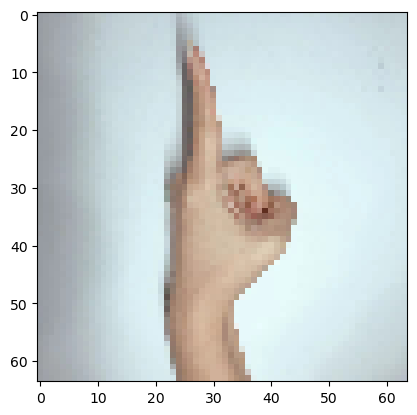
import matplotlib.pyplot as plt # plt 用于显示图片
import matplotlib.image as mpimg # mpimg 用于读取图片
import numpy as np

#这是我女朋友拍的图片
my_image1 = "1.png"                                            #定义图片名称
fileName1 = "C:/Users/TJRA/Desktop/" + my_image1                      #图片地址
image1 = mpimg.imread(fileName1)                               #读取图片
plt.imshow(image1)                                             #显示图片
my_image1 = image1.reshape(1,64 * 64 * 3).T                    #重构图片
my_image_prediction = predict(my_image1, parameters)  #开始预测
print("预测结果: y = " + str(np.squeeze(my_image_prediction)))
预测结果: y = 1
import matplotlib.pyplot as plt # plt 用于显示图片
import matplotlib.image as mpimg # mpimg 用于读取图片
import numpy as np

#这是我女朋友拍的图片
my_image1 = "2.png"                                            #定义图片名称
fileName1 = "C:/Users/TJRA/Desktop/" + my_image1                      #图片地址
image1 = mpimg.imread(fileName1)                               #读取图片
plt.imshow(image1)                                             #显示图片
my_image1 = image1.reshape(1,64 * 64 * 3).T                    #重构图片
my_image_prediction = predict(my_image1, parameters)  #开始预测
print("预测结果: y = " + str(np.squeeze(my_image_prediction)))
预测结果: y = 2
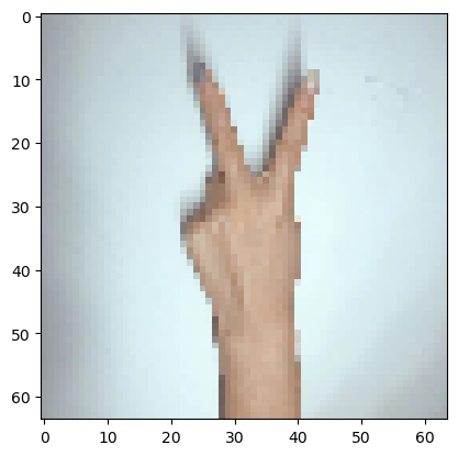
博主拍了六张照片,只对了2张,事实看来,这次的神经网络还有很大的提升空间
相关库代码
#tf_utils.py

import h5py
import numpy as np
import tensorflow as tf
import math

def load_dataset():
    train_dataset = h5py.File('datasets/train_signs.h5', "r")
    train_set_x_orig = np.array(train_dataset["train_set_x"][:]) # your train set features
    train_set_y_orig = np.array(train_dataset["train_set_y"][:]) # your train set labels

    test_dataset = h5py.File('datasets/test_signs.h5', "r")
    test_set_x_orig = np.array(test_dataset["test_set_x"][:]) # your test set features
    test_set_y_orig = np.array(test_dataset["test_set_y"][:]) # your test set labels

    classes = np.array(test_dataset["list_classes"][:]) # the list of classes

    train_set_y_orig = train_set_y_orig.reshape((1, train_set_y_orig.shape[0]))
    test_set_y_orig = test_set_y_orig.reshape((1, test_set_y_orig.shape[0]))

    return train_set_x_orig, train_set_y_orig, test_set_x_orig, test_set_y_orig, classes


def random_mini_batches(X, Y, mini_batch_size = 64, seed = 0):
    """
    Creates a list of random minibatches from (X, Y)

    Arguments:
    X -- input data, of shape (input size, number of examples)
    Y -- true "label" vector (containing 0 if cat, 1 if non-cat), of shape (1, number of examples)
    mini_batch_size - size of the mini-batches, integer
    seed -- this is only for the purpose of grading, so that you're "random minibatches are the same as ours.

    Returns:
    mini_batches -- list of synchronous (mini_batch_X, mini_batch_Y)
    """

    m = X.shape[1]                  # number of training examples
    mini_batches = []
    np.random.seed(seed)

    # Step 1: Shuffle (X, Y)
    permutation = list(np.random.permutation(m))
    shuffled_X = X[:, permutation]
    shuffled_Y = Y[:, permutation].reshape((Y.shape[0],m))

    # Step 2: Partition (shuffled_X, shuffled_Y). Minus the end case.
    num_complete_minibatches = math.floor(m/mini_batch_size) # number of mini batches of size mini_batch_size in your partitionning
    for k in range(0, num_complete_minibatches):
        mini_batch_X = shuffled_X[:, k * mini_batch_size : k * mini_batch_size + mini_batch_size]
        mini_batch_Y = shuffled_Y[:, k * mini_batch_size : k * mini_batch_size + mini_batch_size]
        mini_batch = (mini_batch_X, mini_batch_Y)
        mini_batches.append(mini_batch)

    # Handling the end case (last mini-batch < mini_batch_size)
    if m % mini_batch_size != 0:
        mini_batch_X = shuffled_X[:, num_complete_minibatches * mini_batch_size : m]
        mini_batch_Y = shuffled_Y[:, num_complete_minibatches * mini_batch_size : m]
        mini_batch = (mini_batch_X, mini_batch_Y)
        mini_batches.append(mini_batch)

    return mini_batches

def convert_to_one_hot(Y, C):
    Y = np.eye(C)[Y.reshape(-1)].T
    return Y


def predict(X, parameters):

    W1 = tf.convert_to_tensor(parameters["W1"])
    b1 = tf.convert_to_tensor(parameters["b1"])
    W2 = tf.convert_to_tensor(parameters["W2"])
    b2 = tf.convert_to_tensor(parameters["b2"])
    W3 = tf.convert_to_tensor(parameters["W3"])
    b3 = tf.convert_to_tensor(parameters["b3"])

    params = {"W1": W1,
              "b1": b1,
              "W2": W2,
              "b2": b2,
              "W3": W3,
              "b3": b3}

    x = tf.placeholder("float", [12288, 1])

    z3 = forward_propagation_for_predict(x, params)
    p = tf.argmax(z3)

    sess = tf.Session()
    prediction = sess.run(p, feed_dict = {x: X})

    return prediction

def forward_propagation_for_predict(X, parameters):
    """
    Implements the forward propagation for the model: LINEAR -> RELU -> LINEAR -> RELU -> LINEAR -> SOFTMAX

    Arguments:
    X -- input dataset placeholder, of shape (input size, number of examples)
    parameters -- python dictionary containing your parameters "W1", "b1", "W2", "b2", "W3", "b3"
                  the shapes are given in initialize_parameters
    Returns:
    Z3 -- the output of the last LINEAR unit
    """

    # Retrieve the parameters from the dictionary "parameters"
    W1 = parameters['W1']
    b1 = parameters['b1']
    W2 = parameters['W2']
    b2 = parameters['b2']
    W3 = parameters['W3']
    b3 = parameters['b3']
                                                           # Numpy Equivalents:
    Z1 = tf.add(tf.matmul(W1, X), b1)                      # Z1 = np.dot(W1, X) + b1
    A1 = tf.nn.relu(Z1)                                    # A1 = relu(Z1)
    Z2 = tf.add(tf.matmul(W2, A1), b2)                     # Z2 = np.dot(W2, a1) + b2
    A2 = tf.nn.relu(Z2)                                    # A2 = relu(Z2)
    Z3 = tf.add(tf.matmul(W3, A2), b3)                     # Z3 = np.dot(W3,Z2) + b3

    return Z3

 浙公网安备 33010602011771号