线性回归学习笔记

线性回归

感觉之前学校里上的机器学习的课的内容已经忘的七七八八了，最近打算看吴恩达的机器学习视频再入门一次，同时写个博客记录一下

1. 回归和分类

回归和分类是监督学习的两种类型，对于回归问题，我们需要去预测连续的输出值，也就是通过一个映射函数，将输入映射成连续值输出；而分类问题则是预测离散的输出值，通过映射函数，将输入映射到若干离散的分类。比如房价预测就是一个回归问题，检查良性肿瘤和恶性肿瘤就是一个分类问题
简单来说如果输出值是离散的，那就是分类问题；如果输出值是连续的，那就是回归问题

2. 线性回归

最简单的回归方法就是线性回归，通过一个线性函数\(h_{\theta}(x) = \theta_0 + \theta_1x_1 + \theta_2x_2+...+\theta_nx_n\)，将输入映射成连续输出值
对于只有最简单的只有一个特征的情况，即\(h_{\theta}(x) = \theta_1x\)
考虑这些点：\(X = [1, 2, 3, 4, 5, 6, 7], y = [4, 20, 31, 32, 40, 53, 50]\)
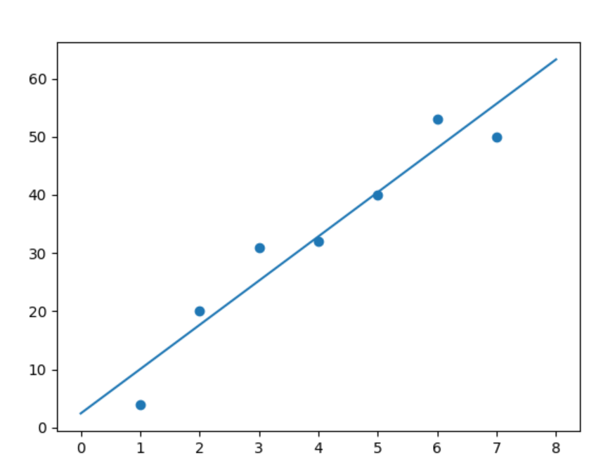
如下图，我们需要找到一个最佳的假设函数去拟合这些点

得到的结果可能就是这样的

（对于一元线性回归，其实就是找一条直线去拟合点）

3. 损失函数

如何判断一个假设函数的好坏，也即如何找到一组\(\theta_i\)，使得期望的预测效果最好
我们定义平方损失函数

\[J(\theta_0,\theta_1,...,\theta_n) = \frac1{2m}\sum_{i=1}^{m}(h_{\theta}(x^{(i)})-y^{(i)})^2 \]

分母上的2只是为了用梯度下降更新参数的时候方便求导
我们的目标就是让平方损失函数最小
首先考虑单变量的情况，即假设

\[h_{\theta}(x) = \theta_1 x \]

选取不同的\(\theta_1\)，得到的平方损失函数值画出来是这样的：

最优点在中间取到，不难理解，拟合度最好的直线肯定不会斜率特别大也不会特别小
而对于双变量的情况，结果应该如下

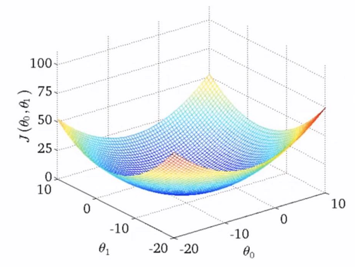
4. 参数调整

为了得到一个比较好的模型，我们需要对参数进行调整，就是找到最优的一组\(\theta_i\)，让平方损失函数最小，即

\[(\theta_0,\theta_1,...,\theta_n)^* = \mathop{\arg\min}\limits_{\theta_0,\theta_1,...,\theta_n} J(\theta_0,\theta_1,...,\theta_n) \]

用的方法就是梯度下降(\(Gradient\ Descent\))
以两个参数的情况为例
初始化\(\theta_0,\theta_1\)
\(J(\theta_0,\theta_1) = \frac1{2m}\sum_{i=1}^{m}(h_{\theta}(x^{(i)})-y^{(i)})^2\)分别对\(\theta_0,\theta_1\)求偏导
然后用偏导数的梯度值更新参数，即

\[\theta_j := \theta_j - \alpha \frac{\partial}{\partial\theta_j}J(\theta_0,\theta_1)\ (for\ j=0\ and\ j=1) \]

\[\frac{\partial}{\partial\theta_j}J(\theta_0,\theta_1) = \frac{\partial}{\partial\theta_j}(\frac1{2m}\sum_{i=1}^{m}(h_{\theta}(x^{(i)})-y^{(i)})^2)=\frac{\partial}{\partial\theta_j}(\frac1{2m}\sum_{i=1}^{m}(\theta_0 + \theta_1x^{(i)}-y^{(i)})^2) \]

最后可以得到：

\[\theta_0 := \theta_0 - \alpha \frac1m\sum_{i=1}^{m} h_{\theta}(x^{(i)})-y^{(i)} \]

\[\theta_1 := \theta_1 - \alpha \frac1m\sum_{i=1}^{m} (h_{\theta}(x^{(i)})-y^{(i)}) * x^{(i)} \]

不断重复上述过程，直至平方损失函数收敛到极小值
其中\(\alpha\)为学习率
要注意的是：学习率过低可能导致收敛速度过慢，学习率过高可能导致参数更新过大从而难以收敛甚至发散，如果选取一个足够小的学习率，是一定能收敛的，但是需要迭代很多次
梯度下降可以用于各种参数优化，但有可能会陷入局部最优解，但是在线性回归中的平方损失函数是一个凸函数，它只有一个局部最大值，也就是局部最大值等于全局最大值，所以最后收敛得到的参数一定是最优的参数组合

5. 一元线性回归

以下是一个最简单的一元线性回归的实现，同时用\(Batch\ grandient\ descent\)来优化参数
如果是多元线性回归的话只要稍微修改一下就可以了

view code

# -*- coding: utf-8 -*-
import numpy as np
from sklearn.datasets import load_boston
import pandas as pd
from sklearn.model_selection import train_test_split
import matplotlib.pyplot as plt

# y = k * x + b
def plot(k, b, color = 'red'):
    x = np.linspace(0,10,100)
    y = k * x + b
    plt.plot(x, y, c = color)

class LinearRegression:
    def __init__(self):
        self.theta0, self.theta1 = 0, 0
        pass
    # 预测函数
    def h(self, x):
        return self.theta0 + self.theta1 * x
    # 计算损失
    def J(self):
        loss = 0
        for i in range(self.m):
            loss += (self.h(self.X[i]) - self.y[i]) ** 2
        return loss / (2 * self.m)

    def fit(self, X, y, theta0 = 0, theta1 = 0, alpha = 10.0, maxiter = 100, eps = .3):
        self.m = X.shape[0]
        self.X = X
        self.y = y
        # 线性回归参数 y = theta0 + theta1 * x
        self.theta0, self.theta1 = theta0, theta1
        lastLoss = -1
        plt.scatter(X,y)
        plot(self.theta1, self.theta0, 'green')
        plt.xlim(xmin = 0, xmax = 9)
        for iterTime in range(maxiter):
            # 梯度
            g0, g1 = 0, 0
            for i in range(self.m):
                g0 += self.h(X[i]) - y[i]
                g1 += (self.h(X[i]) - y[i]) * X[i]
                g0 /= self.m
                g1 /= self.m
            self.theta0 -= alpha * g0
            self.theta1 -= alpha * g1
            nowLoss = self.J()
            if lastLoss != -1 and abs(nowLoss - lastLoss) < eps:
                break
            lastLoss = nowLoss
            plot(self.theta1, self.theta0)
        self.mse = lastLoss
        plt.show()
    def pred(self, X):
        n = X.shape[0]
        y_pred = np.zeros(n)
        for i in range(n):
            y_pred[i] = self.h(X[i])
        return y_pred


if __name__ == '__main__':
    dataset = load_boston()
    X = dataset.data[:,5]
    y = dataset.target
    fname = dataset.feature_names[5]
    # 删除一些偏差过大的数据
    idx = np.where(y!=50)
    X = X[idx]
    y = y[idx]
    X_train, X_test, y_train, y_test = train_test_split(X,y,test_size = 0.4, random_state = 42)
    model = LinearRegression()
    model.fit(X_train,y_train, theta0 = -20, theta1 = 1, alpha = 5, maxiter = 20, eps = 0)
    y_pred = model.pred(X_test)
    print(model.mse)

6. 多元线性回归

\[h_{\theta} = \theta_0 + \theta_1x_1 + \theta_2x_2 + ... + \theta_nx_n = \theta_0 + \sum_{j=1}^n \theta_jx_j \]

\[J(\theta_0,\theta_1,...,\theta_n) = \frac1{2m}\sum_{i=1}^{m}(h_{\theta}(x^{(i)})-y^{(i)})^2 = \frac1{2m}\sum_{i=1}^{m} ((\theta_0 + \sum_{j=1}^n \theta_jx^{(i)}_{j})-y^{(i)})^2 \]

\[\frac{\partial}{\partial \theta_0}J(\theta_0,\theta_1,...,\theta_n) = \frac{1}{m} \sum_{i=1}^m ((\theta_0 + \sum_{j=1}^n \theta_jx^{(i)}_{j}) - y^{(i)}) \]

\[\frac{\partial}{\partial \theta_k}J(\theta_0,\theta_1,...,\theta_n) = \frac{1}{m} \sum_{i=1}^m ((\theta_0 + \sum_{j=1}^n \theta_jx^{(i)}_{j}) - y^{(i)}) x^{(i)}_{k},\ k \ne 0 \]

view code

# -*- coding: utf-8 -*-
import numpy as np
from sklearn.datasets import load_boston
import pandas as pd
from sklearn.model_selection import train_test_split
import matplotlib.pyplot as plt

class LinearRegression:
    def __init__(self):
        pass
    # 预测函数
    def h(self, x):
        H = self.theta[0]
        for i in range(x.shape[0]):
            H += x[i] * self.theta[i-1]
        return H
    # 计算损失
    def J(self):
        mse = 0
        for i in range(self.m):
            mse += (self.h(self.X.iloc[i]) - self.y[i]) ** 2
        return mse / (2 * self.m)

    def fit(self, X, y, theta = None, alpha = 10.0, maxiter = 100, eps = .3):
        self.m = X.shape[0]
        self.n = X.shape[1]
        self.X = X
        self.y = y
        # 线性回归参数 y = theta0 + theta1 * x
        if (theta is not None) and (len(theta) == self.n + 1):
            self.theta = np.array(theta)
        else:
            self.theta = np.zeros((self.n+1,))
        lastMSE = -1
        for iterTime in range(maxiter):
            # 梯度
            g = np.zeros((self.n+1,))
            for i in range(self.m):
                g[0] += self.h(X.iloc[i]) - y[i]
            for j in range(1,self.n+1):
                for i in range(self.m):
                    g[j] += (self.h(X.iloc[i]) - y[i]) * X.iloc[i,j-1]
                g[j] /= self.m
            for i in range(self.theta.shape[0]):
                self.theta[i] -= alpha * g[i]
            curMSE = self.J()
            if lastMSE != -1 and abs(curMSE - lastMSE) < eps:
                break
            lastMSE = curMSE
        self.mse = lastMSE
    def pred(self, X):
        m = X.shape[0]
        y_pred = np.zeros(m)
        for i in range(m):
            y_pred[i] = self.h(X.iloc[i])
        return y_pred


if __name__ == '__main__':
    dataset = load_boston()
    X = dataset.data[:,5]
    y = dataset.target
    fname = dataset.feature_names[5]
    # 删除一些偏差过大的数据
    idx = np.where(y!=50)
    X = X[idx]
    y = y[idx]
    X_train, X_test, y_train, y_test = train_test_split(X,y,test_size = 0.4, random_state = 42)
    dfX_train = pd.DataFrame(X_train)
    dfX_test = pd.DataFrame(X_test)
    model = LinearRegression()
    model.fit(dfX_train,y_train, theta = (0,5), alpha = 0.004, maxiter = 20, eps = 1)
    y_pred = model.pred(dfX_test)
    print(model.mse)

7. 多项式回归

其实多项式回归也是线性回归，只是添加了原来特征的高次项，举个例子：
比如原来的假设函数\(h_{\theta}(x) = \theta_0 + \theta_1 x\)
我们添加特征\(x\)的若干次项，就变成了\(h_{\theta}(x) = \theta_0 + \theta_1 x + \theta_2 x^2 + \theta_3 x^3\)或者\(h_{\theta}(x) = \theta_0 + \theta_1 x + \theta_2 x^2 + \theta_3 \sqrt{x}\)或者其他的
相当于添加了新的特征，然后用多元线性回归去做就好了

注意添加了高次项之后如果要用梯度下降优化参数最好要做归一化处理，否则梯度下降收敛的速度会很慢

8. 正规方程

多元线性回归，也可以写成矩阵形式，同时定义\(x^{(i)}_0 = 1\)
然后用正规方程直接求解最优参数，以下是推导过程（其实就是最小二乘法）：

\[X = \left( \begin{array}{cccc} x^{(1)}_{0} & x^{(1)}_{1} & \cdots & x^{(1)}_{n} \\ x^{(2)}_{0} & x^{(2)}_{1} & \cdots & x^{(2)}_{n} \\ \vdots & \vdots & \ddots & \vdots \\ x^{(m)}_{0} & x^{(m)}_{1} & \cdots & x^{(m)}_{n} \end{array}\right) \]

\[\theta = \left( \begin{array}{c} \theta_0 \\ \theta_1 \\ \vdots \\ \theta_n \end{array}\right) \]

\[y = \left( \begin{array}{c} y^{(1)} \\ y^{(2)} \\ \vdots \\ y^{(m)} \end{array}\right) \]

\[h_{\theta}(X) = X \theta \]

\[J(\theta) = \frac1{2m}(h_{\theta}(X) - y)^T(h_{\theta}(X) - y) = \frac1{2m}(X \theta - y)^T(X \theta - y) \]

\[\frac{\partial}{\partial \theta} J(\theta) = \frac1mX^T(X \theta - y) = 0 \]

\[\hat{\theta} = (X^TX)^{-1}X^Ty \]

view code

import numpy as np
import matplotlib.pyplot as plt
import pandas as pd
from sklearn.metrics import mean_squared_error
import numpy.linalg as alg

class NormalFunctionLinearRegression:
    def __init__(self):
        pass
    def fit(self, X, y):
        m, n = X.shape
        X = np.hstack((np.ones((m,1)),np.array(X)))
        y = np.array(y).reshape((m,1))
        self.theta = alg.inv(X.transpose().dot(X)).dot(X.transpose()).dot(y)
        return np.copy(self.theta)
    def predict(self, X):
        m, n = X.shape
        X = np.hstack((np.ones((m,1)),np.array(X)))
        return X.dot(self.theta)
    pass


if __name__ == '__main__':
    X = np.array([1,2,3,4,5,6,7])
    y = np.array([4,20,31,32,40,53,50])
    model = NormalFunctionLinearRegression()
    X = pd.DataFrame(X)
    theta = model.fit(X, y)
    print(theta)
    plt.scatter(X,y)
    xl = np.linspace(0,8,5)
    yl = theta[0] + theta[1] * xl
    plt.plot(xl,yl)
    plt.show()

那么有了简单便利的正规方程为什么还要用梯度下降呢
其实正规方程和梯度下降各有优缺点

梯度下降需要自己选择学习率\(\alpha\)，而且需要多次迭代
正规方程不需要选择\(\alpha\)，不需要迭代
但是对于特征比较多的情况下，正规方程的求解需要用到矩阵计算，复杂度是\(O(n^3)\)，而梯度下降可以在若干次迭代之后收敛到最优值附近

所以对于不同的任务，可以选取不同的方法

9. 特征缩放 归一化 标准化

如果有多个特征，且各个特征的取值范围差别比较大，那么直接进行梯度下降来找最优解会导致速度过慢。如果先做归一化处理再去做梯度下降会加快收敛速度

通常归一化可以用下式：

\[x^{(i)}_j := \frac{x^{(i)}_j - \mu_j}{s_{j}} \]

其中\(\mu_j\)为第\(j\)个特征的样本均值，\(s_j\)可以为第\(j\)个特征的样本标准差，根据中心极限定律，归一化之后\(x_j\)服从正态分布

也可以用下式：

\[x^{(i)}_j := \frac{x^{(i)}_j - \mu_j}{\max{x_j} - \min{x_j}} \]

其中\(\mu_j\)为第\(j\)个特征的样本均值，\(\max{x_j}、\min{x_j}\)分别式第\(j\)类特征的最大值和最小值

用上面的办法归一化之后各特征符合零均值

如果用正规方程去求解最优解的话是不需要归一化的