MOT相关

核心参考
核心参考：目标跟踪初探（DeepSORT）
核心参考：Sort和Deepsort原理解析及在JDE和Fairmot中的应用

目录

• 核心技术
  • 匈牙利算法（Hungarian Algorithm）
  • 卡尔曼滤波（Kalman Filter）
    • 预测
    • 更新
  • 马氏距离（Mahalanobis Distance）
    • 是什么
    • 解决了什么问题
    • 哪些不足
• 核心步骤
  • 评价指标
  • 数据集 Benchmark
• SORT和DeepSORT
  • SORT
  • DeepSORT
    • 外观特征
    • 马氏距离
• Related Work

核心技术

匈牙利算法（Hungarian Algorithm）

C语言实现，b站视频
匈牙利算法解决的是分配问题，是一个为了解决二分图问题的一种匹配算法，复杂度 \(O(n^3)\) 。使用方法如下

import numpy as np 
from sklearn.utils.linear_assignment_ import linear_assignment
from scipy.optimize import linear_sum_assignment

cost_matrix = np.array([
    [15,40,45],
    [20,60,35],
    [20,40,25]
])
 
matches = linear_assignment(cost_matrix)
print('sklearn API result:\n', matches)
matches = linear_sum_assignment(cost_matrix)
print('scipy API result:\n', matches)

"""Outputs
sklearn API result:
 [[0 1]
  [1 0]
  [2 2]]
scipy API result:
 (array([0, 1, 2], dtype=int64), array([1, 0, 2], dtype=int64))
"""

卡尔曼滤波（Kalman Filter）

B站视频

用于修正传感器的测量值，达到更精确的估计

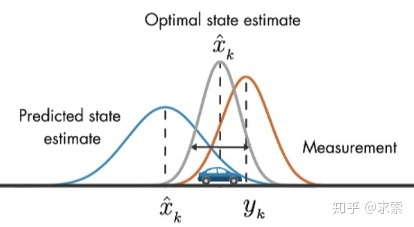
假设我们要跟踪小车的位置变化，如下图所示，蓝色的分布是卡尔曼滤波预测值，棕色的分布是传感器的测量值，灰色的分布就是预测值基于测量值更新后的最优估计。

在目标跟踪中，需要估计track的以下两个状态：

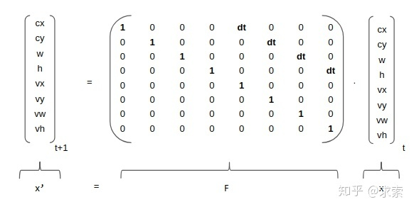
• 均值(Mean)：表示目标的位置信息，由bbox的中心坐标 (cx, cy)，宽高比r，高h，以及各自的速度变化值组成，由8维向量表示为 x = [cx, cy, r, h, vx, vy, vr, vh]，各个速度值初始化为0。
• 协方差(Covariance )：表示目标位置信息的不确定性，由8x8的对角矩阵表示，矩阵中数字越大则表明不确定性越大，可以以任意值初始化。

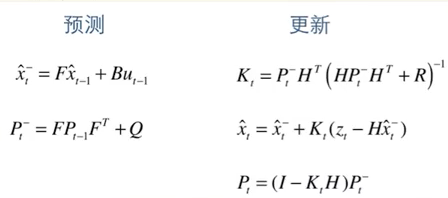
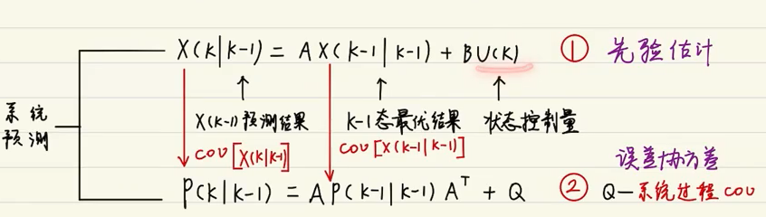
卡尔曼滤波分为两个阶段：(1) 预测track在下一时刻的位置，(2) 基于detection来更新预测的位置。

下面将介绍这两个阶段用到的计算公式。（这里不涉及公式的原理推导，因为我也不清楚原理(ಥ_ಥ) ，只是说明一下各个公式的作用）

预测

基于track在t-1时刻的状态来预测其在t时刻的状态。

当一个小车移动后，且其初始定位和移动过程都是高斯分布时，则最终估计位置分布会更分散，即更不准确
说白话就是，使用k-1态的最优结果，加上k-1态的状态控制量（是否精确取决于系统的运动方程是否精确）

\[x ^ { \prime } = F x \]

\[P ^ { \prime } = F P F ^ { T } + Q \]

其中 \(F\) 为状态转移矩阵， \(P\) 为协方差矩阵， \(Q\) 为噪声矩阵（代表系统可靠性，一般为极小值）。由下图可以发现卡尔马滤波是匀速模型。

#  kalman_filter.py
def predict(self, mean, covariance):
    """Run Kalman filter prediction step.
    
    Parameters
    ----------
    mean: ndarray, the 8 dimensional mean vector of the object state at the previous time step.
    covariance: ndarray, the 8x8 dimensional covariance matrix of the object state at the previous time step.
 
    Returns
    -------
    (ndarray, ndarray), the mean vector and covariance matrix of the predicted state. 
     Unobserved velocities are initialized to 0 mean.
    """
    std_pos = [
        self._std_weight_position * mean[3],
        self._std_weight_position * mean[3],
        1e-2,
        self._std_weight_position * mean[3]]
    std_vel = [
        self._std_weight_velocity * mean[3],
        self._std_weight_velocity * mean[3],
        1e-5,
        self._std_weight_velocity * mean[3]]
    
    motion_cov = np.diag(np.square(np.r_[std_pos, std_vel]))  # 初始化噪声矩阵Q
    mean = np.dot(self._motion_mat, mean)  # x' = Fx
    covariance = np.linalg.multi_dot((self._motion_mat, covariance, self._motion_mat.T)) + motion_cov  # P' = FPF(T) + Q
 
    return mean, covariance

更新

基于t时刻检测到的detection，校正与其关联的track的状态，得到一个更精确的结果。

当一个小车经过传感器观测定位，且其初始定位和观测都是高斯分布时，则观测后的位置分布会更集中，即更准确
说白话就是，通过k态的观测值，与k态估计值，生成k态最优结果，并对相应的矩阵（运动状态方程）进行更新。

\[y = z - H x ^ { \prime } \]

在公式1中，z为detection的均值向量，不包含速度变化值，即z=[cx, cy, r, h]，H称为测量矩阵，它将track的均值向量x'映射到检测空间，该公式计算detection和track的均值误差；

\[S = HP ^ { \prime }H^T + R \]

在公式2中，R为检测器的噪声矩阵，它是一个4x4的对角矩阵，对角线上的值分别为中心点两个坐标以及宽高的噪声，以任意值初始化，一般设置宽高的噪声大于中心点的噪声，该公式先将协方差矩阵P'映射到检测空间，然后再加上噪声矩阵R；

\[K = P^{\prime}H^T S ^ { -1 } \]

公式3计算卡尔曼增益K，卡尔曼增益用于估计误差的重要程度；

\[x = x ^ { \prime } + Ky \]

\[P = ( I - K H ) P ^ { \prime } \]

公式4和公式5得到更新后的均值向量x和协方差矩阵P。

#  kalman_filter.py
def project(self, mean, covariance):
    """Project state distribution to measurement space.

    Parameters
    ----------
    mean: ndarray, the state's mean vector (8 dimensional array).
    covariance: ndarray, the state's covariance matrix (8x8 dimensional).

    Returns
    -------
    (ndarray, ndarray), the projected mean and covariance matrix of the given state estimate.
    """
    std = [self._std_weight_position * mean[3],
           self._std_weight_position * mean[3],
           1e-1,
           self._std_weight_position * mean[3]]

    innovation_cov = np.diag(np.square(std))  # 初始化噪声矩阵R
    mean = np.dot(self._update_mat, mean)  # 将均值向量映射到检测空间，即Hx'
    covariance = np.linalg.multi_dot((
        self._update_mat, covariance, self._update_mat.T))  # 将协方差矩阵映射到检测空间，即HP'H^T
    return mean, covariance + innovation_cov


def update(self, mean, covariance, measurement):
    """Run Kalman filter correction step.

    Parameters
    ----------
    mean: ndarra, the predicted state's mean vector (8 dimensional).
    covariance: ndarray, the state's covariance matrix (8x8 dimensional).
    measurement: ndarray, the 4 dimensional measurement vector (x, y, a, h), where (x, y) is the 
                 center position, a the aspect ratio, and h the height of the bounding box.
    Returns
    -------
    (ndarray, ndarray), the measurement-corrected state distribution.
    """
    # 将mean和covariance映射到检测空间，得到Hx'和S
    projected_mean, projected_cov = self.project(mean, covariance)
    # 矩阵分解（这一步没看懂）
    chol_factor, lower = scipy.linalg.cho_factor(projected_cov, lower=True, check_finite=False)
    # 计算卡尔曼增益K（这一步没看明白是如何对应上公式5的，求线代大佬指教）
    kalman_gain = scipy.linalg.cho_solve(
            (chol_factor, lower), np.dot(covariance, self._update_mat.T).T,
            check_finite=False).T
    # z - Hx'
    innovation = measurement - projected_mean
    # x = x' + Ky
    new_mean = mean + np.dot(innovation, kalman_gain.T)
    # P = (I - KH)P'
    new_covariance = covariance - np.linalg.multi_dot((kalman_gain, projected_cov, kalman_gain.T))

    return new_mean, new_covariance

马氏距离（Mahalanobis Distance）

用于应对高维线性分布的数据中各维度间非独立同分布的问题

是什么

欧氏距离、曼哈顿距离、汉明距离
马氏距离是欧式距离的一种修正，修正了欧式距离中各个维度尺度不一致且相关的问题，可以应对高维线性分布的数据中各维度间非独立同分布的问题。
单个数据点的马氏距离

\[D_{M}(x)=\sqrt{(x-\mu)^{T} \Sigma^{-1}(x-\mu)} \]

数据点x, y之间的马氏距离

\[D_{M}(x, y)=\sqrt{(x-y)^{T} \Sigma^{-1}(x-y)} \]

其中 \(\Sigma\) 是多维随机变量的协方差矩阵，μ为样本均值，如果协方差矩阵是单位向量，也就是各维度独立同分布，马氏距离就变成了欧氏距离。

解决了什么问题

对变量按照主成分进行旋转，使得不同维度之间互相独立，然后进行标准化，一来相当于对不同尺度的信息进行了归一化（均值与方差），二来消除了非独立同分布的问题。

哪些不足

1. 协方差矩阵 \(\Sigma\) 必须满秩，要求数据有个原维度的特征值，如果没有可以考虑先进行PCA（这种情况下不会损失信息）
2. 不能处理非线性流形（manifold）上的问题
   只对线性空间有效，，如果要处理流形，只能在局部定义，可以用来建立KNN图

核心步骤

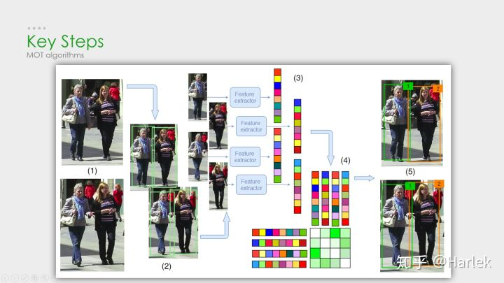
1. 给定视频的原始帧
2. 运行对象检测器以获得对象的边界框
3. 对于每个检测到的物体，计算出不同的特征，一般为视觉特征和动作特征
4. 之后，相似度计算步骤计算两个对象属于同一目标的概率
5. 最后，关联步骤为每个对象分配数字ID

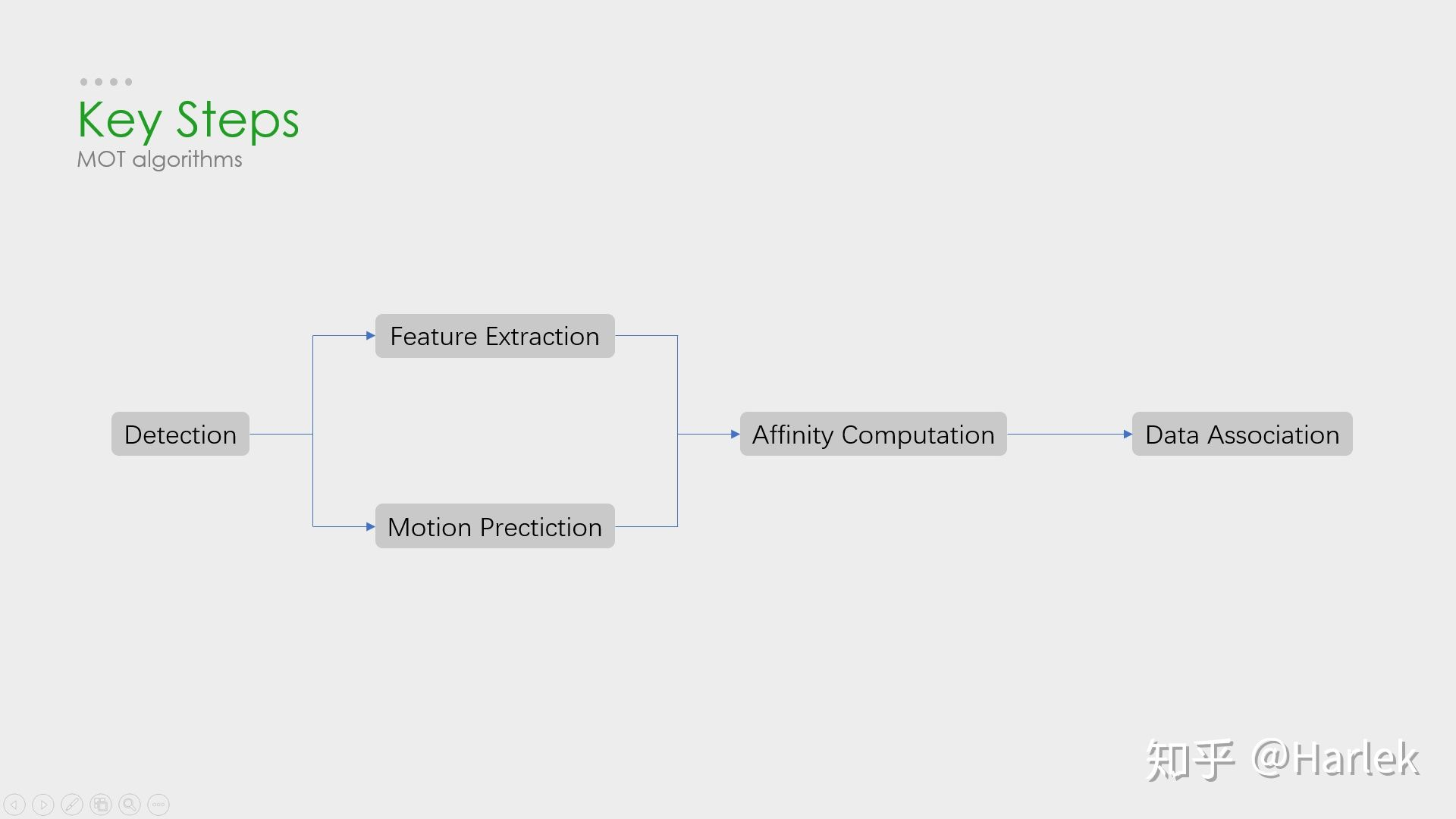
核心步骤：检测——特征提取、运动预测——相似度计算——数据关联
检测所最为重要的部分，对最后指标影响最大。

但是，多目标追踪的研究重点又在相似度计算和数据关联这一块。所以就有一个很大的问题：你设计出更好的关联算法可能就提升了0.1个点，但别人用一些针对数据集的trick消除了一些漏检可能就能涨好几个点。所以研究更好的数据关联的回报收益很低。因此多目标追踪这一领域虽然工业界很有用，但学术界里因为指标数据集的一些原因，入坑前一定要三思。

评价指标

作者首先说明了一个好的tracker应当有两个性质：

• 准确性：能够准确确定目标位置。
• 稳定性：能够持续追踪目标，并且每个目标有唯一轨迹。

因此，评价指标在设计时也要能够反映这两点，另外还应满足：

• 要调的参数少，自适应强。
• 清晰，易懂，直观。
• 普适性强，适用于2D，3D，不同追踪器等。
• 指标数量少，但评价能力强。

1. 记录

2. Clear MOT metrics

\[MOTA =1-\frac{F N+F P+I D S W}{G T} \in(-\infty, 1] \]

\[MOTP =\frac{\Sigma_{t, i} d_{t, i}}{\Sigma_{t} c_{t}} \]

MOTA用的最多，但是FN、FP的权重很大，更多检测的是检测的质量，而不是跟踪的效果

2. IDscores

\[Identification\ precision: IDP=\frac{I D T P}{I D T P+I D F P} \]

\[Identification\ recall: IDR=\frac{I D T P}{I D T P+I D F N} \]

\[Identification\ F1: IDF1 =\frac{2}{\frac{1}{T D P}+\frac{1}{T D R}}=\frac{2 I D T P}{2 I D T P+I D F P+I D F N} \]

因为是基于匹配的指标，能够更好的衡量数据的好坏

数据集 Benchmark

1. MOTChallenge

• 包含
  MOT15（22videos，ACF）
  MOT16（14videos，DPM），
  MOT17（DPM，SDP，Faster R-CNN），
  MOT19（8videos，CVPR19比赛，特别拥挤的场景）
• 使用最多，专注于行人追踪

2. KITTI

• 针对自动驾驶的数据集，MOT中使用较少

3. Other datasets

SORT和DeepSORT

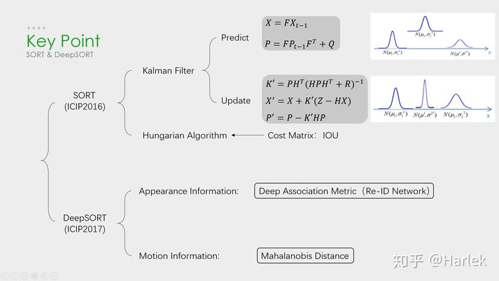
SORT

论文,代码
SORT算法是在卡尔曼滤波的基础上，用匈牙利算法将卡尔曼滤波预测的BBOX与物体检测的BBOX进行了匹配（关联两个BBox的核心算法是：用IOU(交集/并集)计算Bbox之间的距离），选择最优关联结果作为下一时刻的物体跟踪BBOX。

优点	缺点
速度快	对物体遮挡几乎没有处理，导致ID switch很频繁
没有遮挡的情况下准确度很高	有遮挡的情况下准确度很低

DeepSORT

优化了匈牙利算法中的代价矩阵，在IOU Match之前做了一次额外的级联匹配，利用了外观特征和马氏距离

#  tracker.py
def _match(self, detections):
    def gated_metric(racks, dets, track_indices, detection_indices):
        """
        基于外观信息和马氏距离，计算卡尔曼滤波预测的tracks和当前时刻检测到的detections的代价矩阵
        """
        features = np.array([dets[i].feature for i in detection_indices])
        targets = np.array([tracks[i].track_id for i in track_indices]
	# 基于外观信息，计算tracks和detections的余弦距离代价矩阵
        cost_matrix = self.metric.distance(features, targets)
	# 基于马氏距离，过滤掉代价矩阵中一些不合适的项 (将其设置为一个较大的值)
        cost_matrix = linear_assignment.gate_cost_matrix(self.kf, cost_matrix, tracks, 
                      dets, track_indices, detection_indices)
        return cost_matrix

    # 区分开confirmed tracks和unconfirmed tracks
    confirmed_tracks = [i for i, t in enumerate(self.tracks) if t.is_confirmed()]
    unconfirmed_tracks = [i for i, t in enumerate(self.tracks) if not t.is_confirmed()]

    # 对confirmd tracks进行级联匹配
    matches_a, unmatched_tracks_a, unmatched_detections = \
        linear_assignment.matching_cascade(
            gated_metric, self.metric.matching_threshold, self.max_age,
            self.tracks, detections, confirmed_tracks)

    # 对级联匹配中未匹配的tracks和unconfirmed tracks中time_since_update为1的tracks进行IOU匹配
    iou_track_candidates = unconfirmed_tracks + [k for k in unmatched_tracks_a if
                                                 self.tracks[k].time_since_update == 1]
    unmatched_tracks_a = [k for k in unmatched_tracks_a if
                          self.tracks[k].time_since_update != 1]
    matches_b, unmatched_tracks_b, unmatched_detections = \
        linear_assignment.min_cost_matching(
            iou_matching.iou_cost, self.max_iou_distance, self.tracks,
            detections, iou_track_candidates, unmatched_detections)

    # 整合所有的匹配对和未匹配的tracks
    matches = matches_a + matches_b
    unmatched_tracks = list(set(unmatched_tracks_a + unmatched_tracks_b))

    return matches, unmatched_tracks, unmatched_detections

# 级联匹配源码  linear_assignment.py
def matching_cascade(distance_metric, max_distance, cascade_depth, tracks, detections, 
                     track_indices=None, detection_indices=None):
    ...
    unmatched_detections = detection_indice
    matches = []
    # 由小到大依次对每个level的tracks做匹配
    for level in range(cascade_depth):
	# 如果没有detections，退出循环
        if len(unmatched_detections) == 0:  
            break
	# 当前level的所有tracks索引
        track_indices_l = [k for k in track_indices if 
                           tracks[k].time_since_update == 1 + level]
	# 如果当前level没有track，继续
        if len(track_indices_l) == 0: 
            continue
		
	# 匈牙利匹配
        matches_l, _, unmatched_detections = min_cost_matching(distance_metric, max_distance, tracks, detections, 
                                                               track_indices_l, unmatched_detections)
        
	matches += matches_l
	unmatched_tracks = list(set(track_indices) - set(k for k, _ in matches))
    return matches, unmatched_tracks, unmatched_detections

外观特征

外观特征就是通过一个Re-ID的网络提取的，而提取这个特征的过程和NLP里词向量的嵌入过程（embedding）很像，所以后面有的论文也把这个步骤叫做嵌入（起源应该不是NLP，但我第一次接触embedding是从NLP里）。

马氏距离

因为欧氏距离忽略空间域分布的计算结果，所以增加了马氏距离作为运动信息的约束。

\[d ^ { ( 1 ) } ( i , j ) = ( d _ { j } - y _ { i } ) ^ { T } S _ { i } - 1 ( d _ { j } - y _ { i } ) \]

\(dj\)和\(yi\)的空间与分布不同，马氏距离能够改善这一情况。设定一个固定阈值，在阈值之内的被认为是两者关联。但是马氏距离并没有改善长时间遮挡后关联不正确导致的ID switch。

什么是NLP的嵌入过程？

Related Work

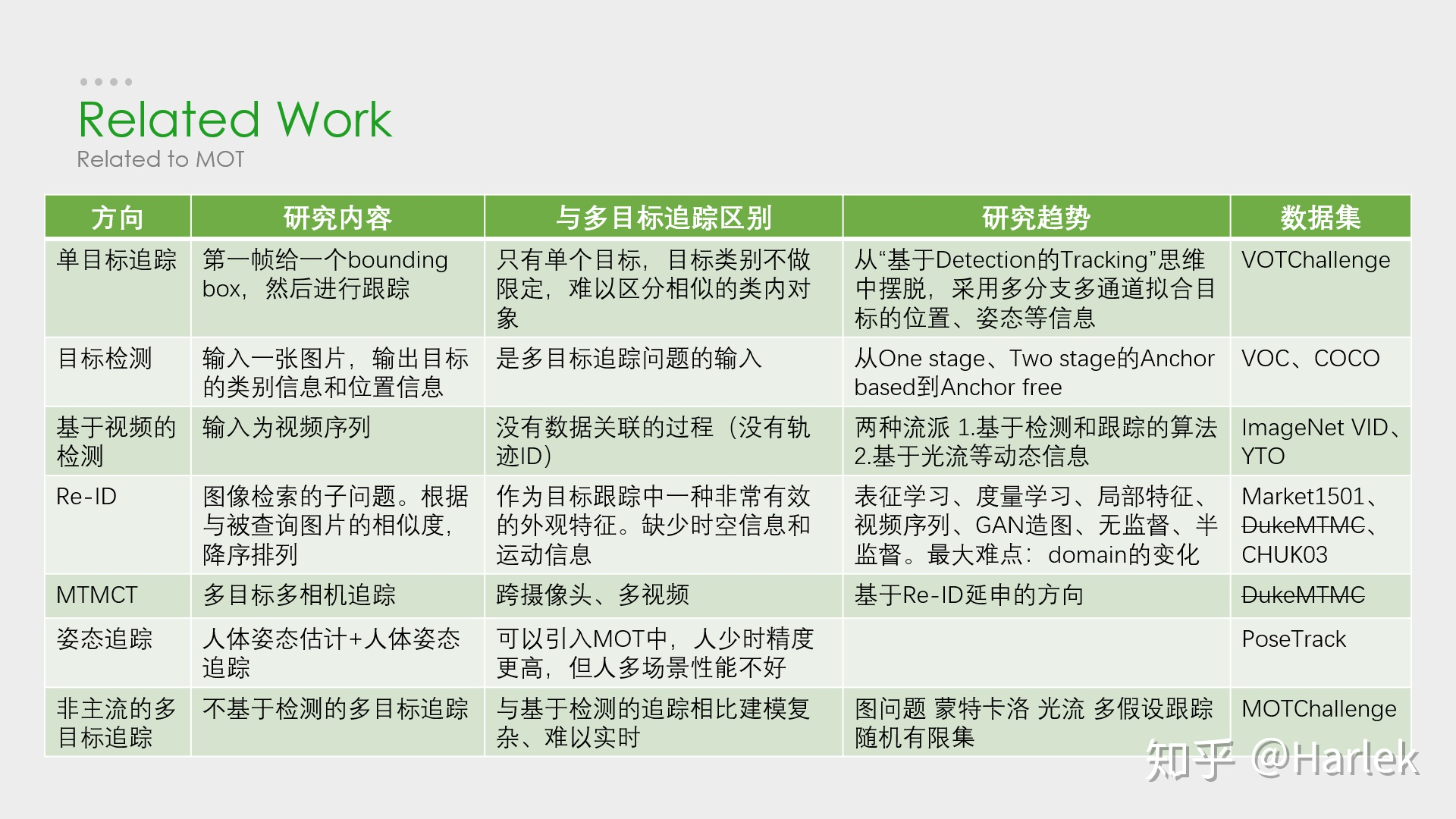
• 单目标追踪，VOT/SOT（hot）
• 目标检测，detection（hot）
• 基于视频的检测
  较为冷门
• 行人重识别，Re-ID（hot）
• 多目标多相机追踪，MTMCT
  因为隐私问题不再提供数据
• 姿态追踪
• 非主流的多目标追踪（不基于检测）