线性系统的频域分析法

Chapter 5 Frequency Domain Analysis Method of Linear System

5-1 Frequency Characteristics

Frequency Characteristics means the frequency response when $\omega$ increases from 0 to $\infin$, and the frequency response of a specific $\omega$ does not represent the dynamic characteristics of the system.

For a system with a transfer function like

$$\Phi(s) = \frac1{Ts+1}$$

when the input is a sine signal like $X\sin\omega t$, it's output is

$$U_i(s) = \frac{X\omega}{s^2+\omega^2}\\ U_C(s) = \frac{X\omega}T\cdot\frac1{(s+\frac1T)(s^2+\omega^2)}$$

The time domain function obtained by the inverse Laplace Transform of this function is quite complicated.

$$u_c(t) = \frac{X\omega T}{T^2\omega^2+1}e^{-\frac1Tt}+\frac{X}{\sqrt{1+T^2\omega^2}}\sin(\omega t-\arctan\omega T)$$

We can easily know that part on the left of plus symbol tends to 0 as time increase. So it's the transient component, and the right part is the steady-state component.

We let steady-state component

$$u_{css}(t) = \frac{X}{\sqrt{1+T^2\omega^2}}\sin(\omega t-\arctan\omega T) = Y\sin(\omega t+\varphi)\\ Y = \frac{X}{\sqrt{1+T^2\omega^2}},\varphi=-\arctan\omega T$$

This means we end up with getting a sine signal in the steady-state component when a sine signal is inputed. Only with amplitude and phase changed, and frequency is not changed.

Follow this thought, we just need to solve $Y$ and $\omega$ before we get the time domain function of output.

Remember when we talked about Laplace Transform, symbol $s$ is defined as $j\omega-\beta$, now we restore it to it's original form and let $\beta =0$ and we get

$$G(j\omega) = \frac1{1+jT\omega}$$

After a careful compare between these formulas we can find out

$$\begin{cases} |G(j\omega)| =\frac YX\\ \angle G(j\omega) = \varphi \end{cases}$$

So once we get a sine signal input and the transfer function of the system, we can quickly calculate the time domain output function of the system, which is quite convenient.

Geometrical representation of frequency characteristics

In engineering analysis and design, the frequency characteristics of the linear system is usually drawn as a curve, and then the graphic method is used for research.

There are three commonly used frequency characteristics curves:

1. Amplitude-Phase frequency characteristics curve --- Nyquist diagram

   The track of $G(j\omega)$ when $\omega$ changes from 0 to $\infin$.

   Nyquist diagram can be drawn in Polar Coordinate System or Cartesian Coordinate System.

2. logarithmic frequency characteristics curve --- Bode diagram (most commonly used)

   Bode diagram is drawn in half logarithmic coordinate system and it actually includes two diagrams: logarithmic amplitude-frequency characteristics curve and logarithmic phase-frequency characteristics curve.

   In amplitude-frequency characteristics curve:

   Horizontal axis: $\omega$

   Vertical axis: $L(\omega) = 20\lg A(\omega) = 20\lg|G(\omega)|$. Unit: dB

   In phase-frequency characteristics curve:

   Horizontal axis: $\omega$

   Vertical axis: $\varphi(\omega)$

3. logarithmic Amplitude-Phase frequency characteristics curve --- Nichols diagram

   Take $\varphi(\omega)$ as horizontal axis, $L(\omega)$ as vertical axis.

5-2 Typical Link and Frequency Characteristics of Open Loop System

The open loop transfer function of the system can usually decomposed into the product of several typical links.

And what's more important: the open-loop frequency characteristics of the system is the synthesis of the frequency characteristics of the typical links that make up the open-loop system.

$$L(\omega) = \sum_{i=1}^NL_i(\omega)\\ \varphi(\omega) = \sum_{i=1}^N\varphi_i(\omega)$$

So here is gonna introduce some typical links which are divided into two groups: minimum-phase links and non-minimum phase links.

You may wonder what is minimum-phase link?

For a closed-loop system, if all of it's open-loop transfer function's poles and zero-points are less or equal 0, then we call the system as minimum-phase system. And if it plays a link in other systems, we call it a minimum-phase link.

1. Minimum-phase links

• proportion link

  $$G(s) = K(K>0)\\ L(\omega) = 20\lg K\\ \varphi(\omega) =0^\circ$$

  $L(\omega)$ is a straight line parallel to $\omega$ axis.

  $\varphi(\omega)$ is a straight line that coincides with the $\omega$ axis.

• integration link

  $$G(s) = \frac1s\\ L(\omega) =-20\lg\omega\\ \varphi(\omega) = -90^\circ$$

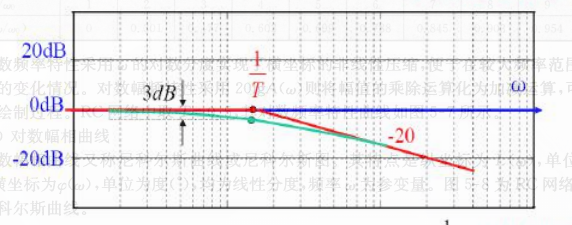
• inertia link

  $$G(s)= \frac1{Ts+1}$$

  Approximately, when $\omega\ll\frac1T, A(\omega)\approx1,L(\omega)\approx 0$

  when $\omega\gg\frac1T, L(\omega)\approx-20(\lg\omega-\lg\frac1T)$. This is a straight line with a slope of -20, and the intersection with $\omega$-axis is $\frac1T$.

  when $\omega=\frac1T, L(\omega)\approx-3dB$

  Approximate diagram:

  

• oscillation link

  $$G(s) = \frac{\omega_n^2}{s^2+2\zeta\omega_ns+\omega_n^2}$$

  for a complex fraction

  $$\frac{a+b\mathrm j}{c+d\mathrm j}$$

  it's module and angle is

  $$module: \sqrt{\frac{a^2+b^2}{c^2+d^2}}\\ angle: \arctan\left(\frac{bc-ad}{ac+bd} \right)$$

  frequency characteristics

  $$A(\omega) = \frac1{\sqrt{\left(1-\dfrac{\omega^2}{\omega_n^2}\right)^2+4\zeta^2\dfrac{\omega^2}{\omega_n^2}}}\\ \begin{align} \varphi(\omega) &= -\arctan\left(\frac{2\zeta\dfrac{\omega}{\omega_n}}{1-\dfrac{\omega^2}{\omega_n^2}} \right) \\&= \begin{cases}-\arctan\dfrac{2\zeta\dfrac\omega{\omega_n}}{1-\dfrac{\omega^2}{\omega_n^2}},\quad\omega\le\omega_n\\-\left(180^\circ-\arctan\dfrac{2\zeta\dfrac{\omega}{\omega_n}}{\dfrac{\omega^2}{\omega_n^2}-1} \right),\quad\omega>\omega_n \end{cases} \end{align}$$

​
​ Apparently, phase-frequency characteristics curve decreases monotonically from $0^\circ$ to $180\circ$.
​
​ However, the amplitude-frequency characteristics curve of oscillation link is not always monotonous. When $0<\zeta\le\sqrt2/2$, the curve increases first and then decreases, so we have to solve it's extreme value. Let
​ $$​ \frac{\mathrm dA(\omega)}{\mathrm d\omega} = 0 ​$$
​ get resonant frequency
​ $$​ \omega_r = \omega_n\sqrt{1-2\zeta^2},\quad0<\zeta\le\frac{\sqrt2}2 ​$$
​ and the resonant peak value
​ $$​ M_r = A(\omega_r) = \frac1{2\zeta\sqrt{1-\zeta^2}} ​$$
​ When $0<\zeta\le\sqrt2/2$, when $\omega\in(0,\omega_r)$, $A(\omega)$ monotonically increases; when $\omega\in(\omega_r,\infin)$, $A(\omega)$ monotonically decreases. And when $\zeta\in(\sqrt2/2,1)$, $A(\omega)$ decreases monotonically.
​

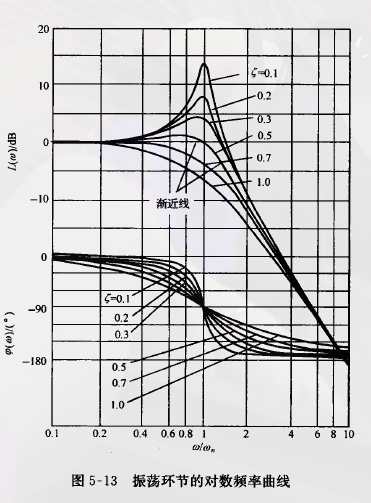
**Notice** that the horizontal axis is not $\omega$ but $\omega/\omega_n$.

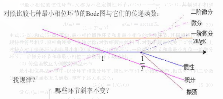
A simple conclusion: If two transfer functions are reciprocal, their Bode diagrams are mirror symmetry about $\omega$-axis.

With this conclusion, we are able to quickly get the figure of pure differential link, first-order differential link and second-order differential link.

• pure differential link

  $G(s) = s$, this is the inverse of integral link.

• first-order differential link

  $G(s) = Ts+1$, the inverse of inertia link.

• second-order differential link

  $G(s) = T^2s^2+2\zeta Ts+1$, the inverse of oscillation link.

2. Non-minimum-phase links

I'm not going to introduce all non-minimum-phase links again. Because for the following links:

• oscillation link
• first-order differential
• second-order differential

their minimum-phase and non-minimum-phase amplitude-frequency characteristics are same, and phase-frequency characteristics have opposite signs which their phase-frequency diagram are symmetrical about $\omega$-axis.

How to draw a rough open-loop amplitude-phase curve

The rough open-loop amplitude-phase curve reflects three important elements of the open-loop frequency characteristics:

• start point($\omega=0$) and end point($\omega=\infin$)
• the intersection with real number axis
• the variation range of the curve (quadrant, monotonicity).

How to draw a Bode diagram

As I said above, a general system can be described as the synthesis of several typical links.

steps:

1. label all the turning frequencies on the diagram;
2. paint low-frequency band characteristics: low-frequency band or it's extension line always pass through the point(1, 20lgK), and it's slope is -20 ;
3. change the slop every time passes a turning frequency;
4. correct all oscillation links and second-order differential links.

Solve transfer function through $L(\omega)$

First, we need to take an another look at this picture:

Let $\omega$ increases from 0, if $L(\omega)$ is a horizontal line at first, then it does not include any differential or integral links. Otherwise it will be an oblique line.

Then, we just need to observe all the points where the slope of the curve changes, if the slope becomes smaller (becomes more steep) after a point, the value of the point on the horizontal axis is the reciprocal of $T$ corresponding to the inertia link; if the slope becomes bigger(less steep) after a point, the values of the point on the horizontal axis is the reciprocal of $T$ corresponding to the first-order differential link.

Last, we just need to solve $K$, which is relatively easy because we know that the curve or it's extension passes through $(1,-20\lg K)$.

5-3 Frequency Domain Stability Criterion

In time domain, there is a Routh Criterion to judge whether the system is stable or not.

In frequency domain, we got Nyquist Stability Criterion and logarithmic Frequency Stability Criterion.

Nyquist Stability Criterion

Let $Z = P-2N$, when Z = 0, the system is stable.

• P: the number of poles
• N: the circle number of $G(j\omega)$ surrounds the point $(-1,j0)$ on G plane.

Argument Principle

Let's say there is a closed curve $\Gamma$ on $s$ plane that surrounds $Z$ zero points and $P$ poles of $F(s)$. If make $s$ move clockwise along the curve $\Gamma$, in $F(s)$ plane, the circles number of the corresponding curve $\Gamma_F$ around the origin is

$$R = P-Z$$

The selection of complex function $F(s)$

$$F(s) = 1+G(s)F(s)$$

Characteristics:

1. Zero points of $F(s)$ are the poles of the closed-loop transfer function, poles of $F(s)$ are the poles of the open-loop transfer function;
2. $F(s)$ has as many zero points and poles;

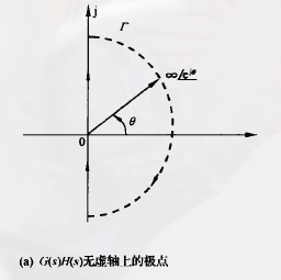
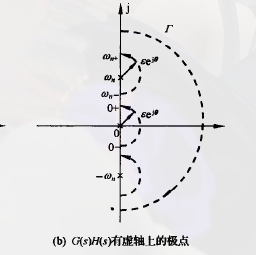
The selection of closed curve $\Gamma$ in $s$ plane

What need to be clear is that $\Gamma$ is not supposed to pass any zero points or poles of $F(s)$.

Under this premise,

• when $F(s)$ has no poles on the imaginary axis

  $\Gamma$ is a semicircle on the right side of the imaginary axis.

  

• when $F(s)$ has poles on the imaginary axis

  Every time a pole is encountered on the imaginary axis, a circle with an infinitely small radius is used to bypass the pole.

  

The determination of turns $\Gamma_F$ around the origin

$$R = 2N = 2(N_+-N_-)$$

Let $N$ be the number of times $\Gamma_{GH}$ crosses the negative real axis to the left of $(-1,j0)$, $N_+$ indicates the number of times when the curve crosses from top to bottom, $N_-$ indicates the number of times when crosses from bottom to top.

Nyquist Stability Criterion Restate

The sufficient and necessary conditions for the stability of a feedback control system are that the semi-closed curve $\Gamma_{GH}$ does not penetrate the point $(-1,j0)$, and the circle number of turns the curve counterclockwise around $(-1,j0)$ $R$ must equal to the number of positive real poles of the open-loop transfer function $P$.

logarithmic Frequency Stability Criterion

(1) The determination of cross points

Let's call the corresponding logarithmic amplitude-frequency curve and the logarithmic phase-frequency curve as $\Gamma_L$ and $\Gamma_\varphi$ in semi-logarithmic coordinate.

When $L(\omega) > 0$, the intersections of $\Gamma_\varphi$ and $(2k+1)\pi(k=0,\pm1,\cdots)$ parallel lines are the cross points we need.

(2) The determination of $\Gamma_{\varphi}$

1. When there is no pole on the imaginary axis, $\Gamma_\varphi$ equals to the $\varphi(\omega)$ curve.

2. When there are integral links $\displaystyle{\frac1{s^\upsilon}}(\upsilon>0)$ exist in the open-loop system. The curve $\Gamma_{GH}$ in the complex plane, need to fill a dotted arc with $\upsilon\times90^\circ$ and an infinite radius from the point $G(j0_+)H(0_+)$. Correspondingly, need to fill a dotted straight line with $\upsilon\times90^\circ$ value in the logarithmic phase-frequency characteristics diagram. The $\varphi(\omega)$ and the supplemented dotted line constructs the $\Gamma_\varphi$.

3. Cross times counting

   positive cross once: when $L(\omega) >0$, $\Gamma_\varphi$ crosses $(2k+1)\pi$ line from bottom to top once;

   negative cross once: when $L(\omega) >0$, $\Gamma_\varphi$ crosses $(2k+1)\pi$ line from top to bottom once;

   positive cross a half time: when $L(\omega)>0$, $\Gamma_\varphi$ from bottom to top starts or from top to bottom ends at $(2k+1)\pi$ line;

   negative cross a half time: when $L(\omega)>0$, $\Gamma_\varphi$ from top to bottom starts or from bottom to top ends at $(2k+1)\pi$ line;

Logarithmic frequency stability criterion: Set $P$ as the number of poles with positive real part, the sufficient and necessary conditions for the feedback control system to stay stable are that when $\varphi(\omega_c)\ne(2k+1)\pi(k=0,1,2,\cdots)$ and $L(\omega)>0$, the times of $\Gamma_\varphi$ crosses the $(2k+1)\pi$ lines

$$N = N_+-N_-$$

satisfy

$$Z = P-2N= 0$$

Logarithmic Frequency Stability Criterion is essentially an expression of Nyquist Stability Criterion under Bode diagram.

5-4 Stability Margin

According to the Nyquist Stability Criterion we know that, the closed-loop stability of the system depends on the turns $\Gamma_{GH}$ around the $(-1,jo)$ when there are poles exist in the right half of the $s$ plane.

However, when some coefficients changed in the open-loop transfer function, the station of $\Gamma_{GH}$ surrounding the $(-1,j0)$ is also changed.

Therefore, in engineering applications, we use phase margin $\gamma$ and magnitude margin $h$ to measure the stability of a system.

1. Phase Margin $\gamma$

Set $\omega_c$ as the system's cut-off frequency, which satisfies

$$A(\omega_c) = |G(j\omega_c)H(j\omega_c) |=1$$

define phase margin as

$$\gamma = 180^\circ+\angle G(j\omega_c)H(j\omega_c)$$

the meaning of the phase margin: for a closed-loop stable system, if the open-loop phase-frequency of the system delays $\gamma$ degree, the system will fall into critical stable state.

2. Magnitude Margin $h$

Set $\omega_x$ as the crossing frequency of the system, then

$$\varphi(\omega_x) = \angle G(j\omega_x)H(j\omega_x) = (2k+1)\pi\quad k=0,\pm1,\cdots$$

define magnitude margin as

$$h =\dfrac1{|G(j\omega_x)H(j\omega_x)|}$$

the meaning of the magnitude margin: for a closed-loop system, if the system's open-loop amplitude-frequency characteristics increases $h$ times, the system will fall into critical stable state.

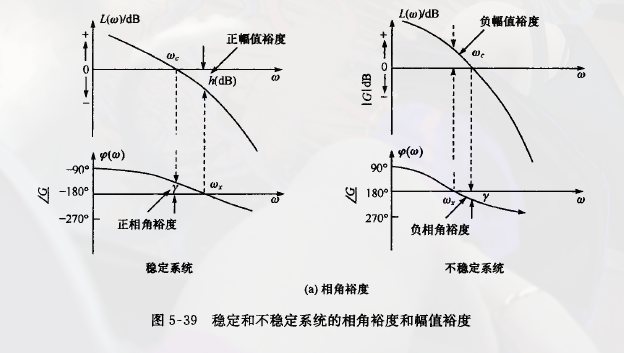
when magnitude margin is presented in dB, if $h>1$, the magnitude margin is a positive value and the system is stable; if $h<1$, the magnitude margin is a negative value and the system is unstable.

The magnitude margin of the first-order system or second-order system is infinity, because the polar coordinate plots of this kind of systems do not intersect with the negative real axis, which means the two systems are impossibly unstable.

Note that for stable systems with two or more cut-off frequencies, magnitude should be calculated at the highest cut-off frequency.

3. Several explanations on phase margin and magnitude margin

Neither the phase margin alone nor the magnitude margin alone is sufficient to explain the stability of the system. In order to determine the stability of the system, two factors must be given simultaneously.

...

5-5 Frequency Domain Performance Indexes of Closed-Loop System

The frequency domain performance indexes of the control closed-loop system should reflect the ability of the control system to track the input signal and suppress interference signals.

1. The Frequency Bandwidth of the Control System

Set $\Phi(\omega)$ as the closed-loop frequency characteristics of the system, when $L(\omega)$ decreases to 3 decibels under the $L(j0)$, the corresponding frequency $\omega_0$ is called the bandwidth frequency. Which means when $\omega>\omega_0$

$$20\lg|\Phi(j\omega)|<20\lg|\Phi(j0)|-3$$

And the frequency range $(0,\omega_0)$ is called the frequency bandwidth. The definition of the bandwidth shows that, for sine input signals with higher frequency than the bandwidth frequency $\omega_0$, the output of the system will present a large attenuation.

For the first-order system:

$$\omega_0 = \frac1T$$

For the second-order system:

$$\omega_0 = \omega_n\sqrt{(1-2\zeta^2)+\sqrt{(1-2\zeta^2)^2+1}}$$

We can see, the bandwidth frequency of the second-order system is proportional to the natural frequency $\omega_n$. And the response speed of the unit step input signal is also proportional to the bandwidth. If the bandwidth of the system is expanded by $\lambda$ times, the response speed of the system is accelerated by $\lambda$ times.

4. The Transformation of the Frequency Domain Indexes and the Time Domain Indexes of the Closed-Loop System

The phase margin $\gamma$ and the cut-off frequency are often used in engineering to estimate the frequency domain performance indexes of the system.

(1) The relationship of the closed-loop and the open-loop frequency domain indexes of the system

Under normal circumstances, around the maximum of $M(\omega)$, there are only small changes in $\gamma(\omega)$, and the resonant frequency $\omega_r$ which makes $M(\omega_r)$ a maximum is normally around the cut-off frequency $\omega_c$.

$$M_r \approx \frac1{|\sin\gamma|}$$

(2) The relationship of the open-loop frequency domain indexes and time domain indexes

$$\gamma = \arctan\frac{2\zeta\omega_n}{\omega_c} = \arctan[2\zeta(\sqrt{4\zeta^4+1}-2\zeta^2)^{-\frac12}]$$

When $\gamma$ is selected, determine $\zeta$ through $\gamma-\zeta$ curve, and then determine $\sigma\%$ and $t_s$ through $\zeta$.