DIN 和 DeepFM 精排模型原理及 Torch-RecHub 代码实战
精排是推荐系统中最重要的环节,也是离用户最近的环节,而 CTR 是评价精排模型性能的重要指标。

CTR,即点击通过率,是互联网广告常用的术语,指网络广告(图片广告/文字广告/关键词广告/排名广告/视频广告等)的点击到达率。CTR 是衡量互联网广告效果的一项重要指标,使用该广告的实际点击次数除以广告的展现量来计算。
本文将介绍提高 CTR 预测的两个经典精排模型 DIN 和 DeepFM,并使用 Torch-RecHub 框架来完成这两个模型的训练和测试。
1. Deep Interest Network (DIN)
1.1 场景和过往研究
CTR 预测 是在线广告等工业应用中的一项基本且重要的任务。基于深度学习的预测模型已经成为了主流,而该模型遵循类似的 Embedding & MLP 范式。在这个范式中,大规模稀疏输入特征(与最终的点击结果可能有关的特征)首先映射为低维嵌入向量,然后以分组方式转换为固定长度的向量,最后连接在一起,输入到多层感知器(MLP)中,学习特征之间的非线性关系,最终输出二分类的结果,如下图所示。在这种方法中,不管候选广告是什么,用户特征都会被压缩成一个固定长度的表示向量。

然而,过往模型存在的问题是无法表达用户广泛的兴趣,因为这些模型在得到各个特征的 embedding 之后,就蛮力拼接和各种交叉等,根本没有考虑之前用户历史行为商品具体是什么。虽然扩大 Embedding 的维度可能增强表达能力,但会快速增加计算的复杂度,在实际中是不可取的。而且,过往模型无法得知用户历史行为中的哪个会对当前的点击预测带来积极的作用,没有权重的区分,如下所示:
假设广告中的商品是键盘,如果用户历史点击的商品中有化妆品,包包,衣服,洗面奶等商品,那么大概率上该用户可能是对键盘不感兴趣的,而如果用户历史行为中的商品有鼠标,电脑,iPad,手机等,那么大概率该用户对键盘是感兴趣的,而如果用户历史商品中有鼠标,化妆品,T-shirt和洗面奶,鼠标这个商品 embedding 对预测“键盘”广告的点击率的重要程度应该大于后面的那三个。
因此,在业务的角度,我们应该自适应的去捕捉用户的兴趣变化,考虑用户的历史行为商品与当前商品广告的一个关联性。基于这个思想,DIN 被提出,在传统模型基础上引入了注意力机制。
1.2 DIN 模型的原理
DIN 引入了一个新的模块,即 local activation unit,能够根据用户历史行为特征和当前广告的相关性给用户历史行为特征 embedding 进行加权。
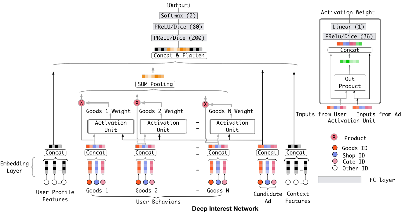
local activation unit 里面是一个前馈神经网络,输入是用户历史行为商品(Key,Value)和当前的候选商品广告(Query),输出是它俩之间的相关性,这个相关性相当于每个历史商品的权重,把这个权重与原来的历史行为 embedding 相乘求和就得到了用户当前的兴趣表示。
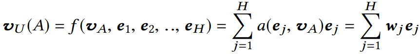
注意:这里的权重加和不是 1,准确的说这里不是权重,而是直接算的相关性的那种分数作为了权重,也就是平时的那种 scores(softmax之前的那个值),这个是为了保留用户的兴趣强度。
1.3 DIN 模型的优势
通过性能比较,DIN 模型在两个数据集上优于其他模型,包括本文也要介绍的 DeepFM,如下所示:

不过也能发现,最好的几个模型的性能都差不多,都是在 1% 级别上做改进。不过对于大规模的业务量来说,这种小的提升就可以带来巨大的利润。
另外,在论文原文中,作者还可视化了不同历史商品的注意力分数,如下所示:

可以发现,上衣类的历史商品(与目标商品较为相似)会有较高的注意力分数,符合人的直觉,表示该模型除了性能更高外,还具备更好的可解释性。
1.4 Amazon 实战案例
1.4.1 任务和数据介绍
实战使用的数据集是 Amazon-Electronics 2014,包括评论(评分、文本、帮助投票)、产品元数据(描述、类别信息、价格、品牌和图像特征) 和链接(查看),共计19万用户、6万商品的信息。官方原数据是 json 格式,可以从以下链接 https://cowtransfer.com/s/e911569fbb1043 下载已经预处理为仅包含 user_id, item_id, cate_id, time 四个特征列的全量 CSV 文件。
该数据集描述了所有用户的历史评论行为(本案例将评论近似于购买行为,因为只有购买才能评论),但要注意很多购买商品的用户并不一定会评论。鉴于难以获取真正的购买行为数据,很多研究包括本文只能使用这种公开数据集进行模拟,测试模型。
任务描述:已知用户过去的商品购买(评论)行为,预测该用户购买(评论)另外一种商品的可能性(在本文中,用0/1的标签表示预测和真实结果,即经典的二分类问题)。
1.4.2 数据载入和预处理
首先,要载入相关的库,并固定随机数种子便于复现
# 检查torch的安装以及 gpu 的使用
import torch
print(torch.__version__, torch.cuda.is_available())
# Output: 1.11.0 False

import torch_rechub # 开发中的推荐算法库
import pandas as pd
import numpy as np
import tqdm
import sklearn

torch.manual_seed(2022) #固定随机种子
然后,载入全量的实验数据。要注意,下面的 file_path 要根据自己的数据文件位置设置,而不是照抄。另外,由于全量数据集有近170万,实验时间较长,于是本文只抽取前 10000 个样本进行案例展示。
# 查看文件
file_path = '../examples/ranking/data/amazon-electronics/amazon_electronic_datasets.csv'
data = pd.read_csv(file_path)
data = data.iloc[:10000,]
data

其中,time 的值越大,说明时间越晚,不同 time 之间的差值单位是 秒。
1.4.3 特征工程
对于模型来说,输入和输出有既定的格式,必须严格执行。对于不同类型的特征,模型也会有不同的预处理和使用方式。在实战中,我们要做的只是告诉模型输入特征所属的类别即可。
- Dense特征:又称数值型特征,例如薪资、年龄,本文暂时没有用到这个类型的特征。
- Sparse特征:又称类别型特征,例如性别、学历。本文对 Sparse 特征直接进行 LabelEncoder 编码操作,将原始的类别字符串映射为数值,在模型中将为每一种取值生成 Embedding 向量。
- Sequence特征:序列特征,比如用户历史点击item_id序列、历史商铺序列等,序列特征如何抽取,是我们在DIN中学习的一个重点,也是DIN主要创新点之一。
在原始数据中是不存在序列特征的,只有用户在不同时刻的行为记录。我们首先需要把这些具有序列特征的行为转换为序列类特征。
from torch_rechub.utils.data import create_seq_features

# 构建用户的历史行为序列特征,内置函数create_seq_features只需要指定数据,和需要生成序列的特征,drop_short是选择舍弃行为序列较短的用户
train, val, test = create_seq_features(data, seq_feature_col=['item_id', 'cate_id'], drop_short=3)

print(len(train), len(val), len(test))
# Output: 60 34 34

# 查看当前构建的序列,在这个案例中我们创建了历史点击序列,和历史类别序列
train
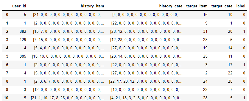
其中,history_item 和 history_cate 就是转换后的序列特征,具有相同的长度,其中的 Id 对应于某个商品或类别,顺序表示行为发生的时间前后关系。Target_item 和 Target_cate 是目标商品广告。Label 表示是否该用户点击了目标广告,1 代表点击,0 代表未点击,这也是 CTR 任务要预测的值。要注意的是,Label 为 0 的样本是自动生成的,而不是原始数据中存在的,具体生成的方法将在本文的 1.5 中介绍。
另外,要注意的是,create_seq_features 方法目前不能按比例去划分训练集、验证集和测试集。若有这方面的需求,可以人为去构造。至于该方法怎么生成的各个数据及,也将在本文的 1.5 中介绍。
1.4.4 模型-特征配置
在这一步,我们需要让模型明白如何处理每一类特征。对于类别特征,我们希望模型将其输入 Embedding 层,而对于序列特征,我们不仅希望模型将其输入Embedding层,还需要计算target-attention分数,所以需要指定DataFrame中每一列的含义,让模型能够正确处理。
在 torch-rechub 我们只需要调用 DenseFeature, SparseFeature, SequenceFeature 这三个类,就能自动正确处理每一类特征。
from torch_rechub.basic.features import DenseFeature, SparseFeature, SequenceFeature

n_users, n_items, n_cates = data["user_id"].max(), data["item_id"].max(), data["cate_id"].max()  # 提取类别数量,这会影响词典的大小

# 这里指定每一列特征的处理方式,对于sparsefeature,需要输入embedding层,所以需要指定特征空间大小和输出的维度;+ 的第一个 1 是因为把 0 作为 Mask 了,+ 的第二个 1 是空出来一位冗余,这是编程习惯问题(猜测是为了新用户商品准备)
features = [SparseFeature("target_item", vocab_size=n_items + 2, embed_dim=8),
            SparseFeature("target_cate", vocab_size=n_cates + 2, embed_dim=8),
            SparseFeature("user_id", vocab_size=n_users + 2, embed_dim=8)]
target_features = features  # target_features 和 features 相同,但为什么要使用不同的变量存储?

# 对于序列特征,除了需要和类别特征一样处理以外,item序列和候选item应该属于同一个空间,我们希望模型共享它们的embedding,所以可以通过shared_with参数指定
history_features = [
    SequenceFeature("history_item", vocab_size=n_items + 2, embed_dim=8, pooling="concat", shared_with="target_item"),
    SequenceFeature("history_cate", vocab_size=n_cates + 2, embed_dim=8, pooling="concat", shared_with="target_cate")]
在上述步骤中,我们制定了每一列的数据如何处理、数据维度、embed后的维度,目的就是在构建模型中,让模型知道每一层的参数。其中,embded_dim 参数是可以改变的,通过参数调整寻找最优值。其他参数一般不用改变。
1.4.5 训练数据生成
对于 1.4.3 生成的三类数据集,我们需要分离 x 和 y,而且要将其转换为 dict 结构(原本为 dataframe)。
from torch_rechub.utils.data import df_to_dict, DataGenerator

# 指定label,生成模型的输入,这一步是转换为字典结构
train = df_to_dict(train)
val = df_to_dict(val)
test = df_to_dict(test)

train_y, val_y, test_y = train["label"], val["label"], test["label"]

# 删除 label 列
del train["label"]
del val["label"]
del test["label"]
train_x, val_x, test_x = train, val, test

# 构建dataloader,指定模型读取数据的方式,和区分验证集测试集、指定batch大小
dg = DataGenerator(train_x, train_y)
train_dataloader, val_dataloader, test_dataloader = dg.generate_dataloader(x_val=val_x, y_val=val_y, x_test=test_x, y_test=test_y, batch_size=16)

# 最后查看一次输入模型的数据格式
train_x

1.4.6 训练和测试
from torch_rechub.models.ranking import DIN
from torch_rechub.trainers import CTRTrainer

# 定义模型,模型的参数需要我们之前的feature类,用于构建模型的输入层,mlp指定模型后续DNN的结构,attention_mlp指定attention层的结构
model = DIN(features=features, history_features=history_features, target_features=target_features, mlp_params={"dims": [256, 128]}, attention_mlp_params={"dims": [256, 128]})  # 这里的 features = target_features,理论上是不合理的,是为了特征太少来凑数?

# 模型训练,需要学习率、设备等一般的参数,此外我们还支持earlystoping策略,及时发现过拟合
ctr_trainer = CTRTrainer(model, optimizer_params={"lr": 1e-3, "weight_decay": 1e-3}, n_epoch=3, earlystop_patience=4, device='cpu', model_path='./')
ctr_trainer.fit(train_dataloader, val_dataloader)

# 查看在测试集上的性能
auc = ctr_trainer.evaluate(ctr_trainer.model, test_dataloader)
print(f'test auc: {auc}')
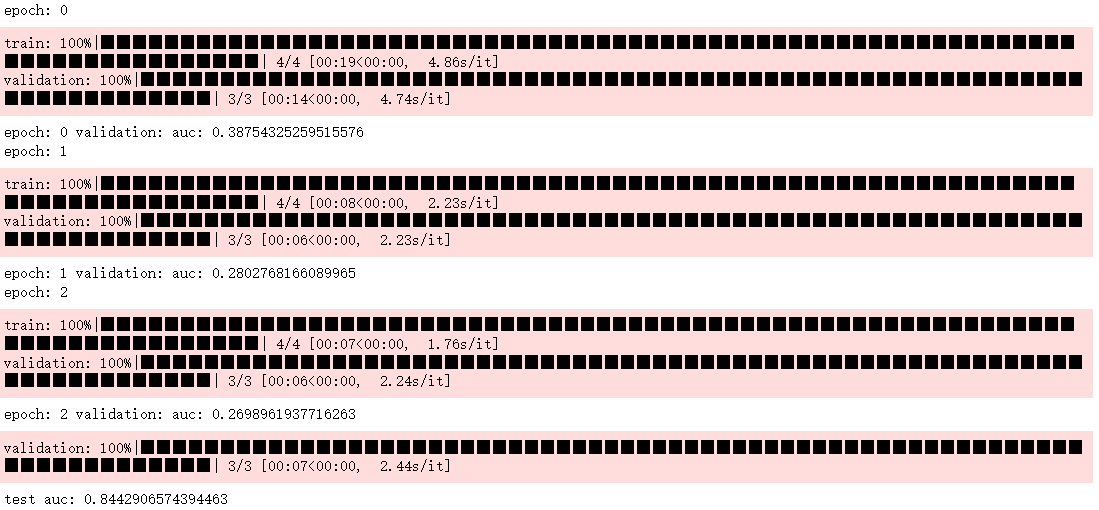
可能是因为数据集规模还是太小,输出的结果有些奇怪。后续应该尝试使用更大规模的数据、更大的Epoch进行训练。
1.5 重要源码的解析
create_seq_features 包含训练、验证和测试集的划分,以及负样本的生成。这部分对模型训练的影响较大,有必要理解其原理。DIN 是核心模型,不管是使用还是改进,都有必要理解其源码,特别是注意力模块。
1.5.1 create_seq_features
源码如下所示,本文将对一些重要语句进行注释。
def create_seq_features(data, seq_feature_col=['item_id', 'cate_id'], max_len=50, drop_short=3, shuffle=True):
    """Build a sequence of user's history by time.

    Args:
        data (pd.DataFrame): must contain keys: `user_id, item_id, cate_id, time`.
        seq_feature_col (list): specify the column name that needs to generate sequence features, and its sequence features will be generated according to userid.
        max_len (int): the max length of a user history sequence.
        drop_short (int): remove some inactive user whose sequence length < drop_short.
        shuffle (bool): shuffle data if true.

    Returns:
        train (pd.DataFrame): target item will be each item before last two items.
        val (pd.DataFrame): target item is the second to last item of user's history sequence.
        test (pd.DataFrame): target item is the last item of user's history sequence.
    """
    for feat in data:
        le = LabelEncoder()
        data[feat] = le.fit_transform(data[feat])
        data[feat] = data[feat].apply(lambda x: x + 1)  # 0 to be used as the symbol for padding
    data = data.astype('int32')

    n_items = data["item_id"].max()

    item_cate_map = data[['item_id', 'cate_id']]
    item2cate_dict = item_cate_map.set_index(['item_id'])['cate_id'].to_dict()

    data = data.sort_values(['user_id', 'time']).groupby('user_id').agg(click_hist_list=('item_id', list), cate_hist_hist=('cate_id', list)).reset_index()

    # Sliding window to construct negative samples
    train_data, val_data, test_data = [], [], []
    for item in data.itertuples():
        if len(item[2]) < drop_short: # drop_short 很关键,如果太小,可能会导致一个样本只会被划分为训练集和测试集,缺少验证集
            continue
        user_id = item[1]
        click_hist_list = item[2][:max_len]
        cate_hist_list = item[3][:max_len]

        neg_list = [neg_sample(click_hist_list, n_items) for _ in range(len(click_hist_list))]
        # 对于每一个样本,随机生成一个同长度的历史序列(有可能与原序列相同,理论上应该避免,但为了降低计算成本,未进行处理;据说不会影响结果),并设置 label 为 0

        hist_list = []
        cate_list = []
        for i in range(1, len(click_hist_list)):
            hist_list.append(click_hist_list[i - 1])
            cate_list.append(cate_hist_list[i - 1])
            hist_list_pad = hist_list + [0] * (max_len - len(hist_list))
            cate_list_pad = cate_list + [0] * (max_len - len(cate_list))
            if i == len(click_hist_list) - 1:
                test_data.append([user_id, hist_list_pad, cate_list_pad, click_hist_list[i], cate_hist_list[i], 1])   # i 表示 target,这也是为什么循环从 1 开始的原因
                test_data.append([user_id, hist_list_pad, cate_list_pad, neg_list[i], item2cate_dict[neg_list[i]], 0])  # 负样本同时生成,这意味着正负样本的数量是相等的
            if i == len(click_hist_list) - 2:
                val_data.append([user_id, hist_list_pad, cate_list_pad, click_hist_list[i], cate_hist_list[i], 1])
                val_data.append([user_id, hist_list_pad, cate_list_pad, neg_list[i], item2cate_dict[neg_list[i]], 0])
            else:
                train_data.append([user_id, hist_list_pad, cate_list_pad, click_hist_list[i], cate_hist_list[i], 1])  # 滑动窗口的处理方式,如果一个用户的历史序列很长,可以生成很多样本(不等长)
                train_data.append([user_id, hist_list_pad, cate_list_pad, neg_list[i], item2cate_dict[neg_list[i]], 0])

    # shuffle
    if shuffle:
        random.shuffle(train_data)
        random.shuffle(val_data)
        random.shuffle(test_data)

    col_name = ['user_id', 'history_item', 'history_cate', 'target_item', 'target_cate', 'label']
    train = pd.DataFrame(train_data, columns=col_name)
    val = pd.DataFrame(val_data, columns=col_name)
    test = pd.DataFrame(test_data, columns=col_name)

    return train, val, test
如果想控制训练集、验证集和测试集遵循一定比例,可以在该方法执行完后,按照比例随机采样。
1.5.2 DIN
class DIN(nn.Module):
    """Deep Interest Network
    Args:
        features (list): the list of `Feature Class`. training by MLP. It means the user profile features and context features in origin paper, exclude history and target features.
        history_features (list): the list of `Feature Class`,training by ActivationUnit. It means the user behaviour sequence features, eg.item id sequence, shop id sequence.
        target_features (list): the list of `Feature Class`, training by ActivationUnit. It means the target feature which will execute target-attention with history feature.
        mlp_params (dict): the params of the last MLP module, keys include:`{"dims":list, "activation":str, "dropout":float, "output_layer":bool`}
        attention_mlp_params (dict): the params of the ActivationUnit module, keys include:`{"dims":list, "activation":str, "dropout":float, "use_softmax":bool`}
    """

    def __init__(self, features, history_features, target_features, mlp_params, attention_mlp_params):
        super().__init__()
        self.features = features
        self.history_features = history_features
        self.target_features = target_features
        self.num_history_features = len(history_features)
        self.all_dims = sum([fea.embed_dim for fea in features + history_features + target_features])

        self.embedding = EmbeddingLayer(features + history_features + target_features)
        self.attention_layers = nn.ModuleList(
            [ActivationUnit(fea.embed_dim, **attention_mlp_params) for fea in self.history_features])
        self.mlp = MLP(self.all_dims, activation="dice", **mlp_params)

    def forward(self, x):
        embed_x_features = self.embedding(x, self.features)  #(batch_size, num_features, emb_dim)
        embed_x_history = self.embedding(
            x, self.history_features)  #(batch_size, num_history_features, seq_length, emb_dim)
        embed_x_target = self.embedding(x, self.target_features)  #(batch_size, num_target_features, emb_dim)
        attention_pooling = []
        for i in range(self.num_history_features):
            attention_seq = self.attention_layers[i](embed_x_history[:, i, :, :], embed_x_target[:, i, :])
            attention_pooling.append(attention_seq.unsqueeze(1))  #(batch_size, 1, emb_dim)
        attention_pooling = torch.cat(attention_pooling, dim=1)  #(batch_size, num_history_features, emb_dim)

        mlp_in = torch.cat([
            attention_pooling.flatten(start_dim=1),
            embed_x_target.flatten(start_dim=1),
            embed_x_features.flatten(start_dim=1)
        ],
                           dim=1)  #(batch_size, N)

        y = self.mlp(mlp_in)
        return torch.sigmoid(y.squeeze(1))


class ActivationUnit(nn.Module):
    """Activation Unit Layer mentioned in DIN paper, it is a Target Attention method.

    Args:
        embed_dim (int): the length of embedding vector.
        history (tensor):
    Shape:
        - Input: `(batch_size, seq_length, emb_dim)`
        - Output: `(batch_size, emb_dim)`
    """

    def __init__(self, emb_dim, dims=[36], activation="dice", use_softmax=False):
        super(ActivationUnit, self).__init__()
        self.emb_dim = emb_dim
        self.use_softmax = use_softmax
        self.attention = MLP(4 * self.emb_dim, dims=dims, activation=activation)

    def forward(self, history, target):
        seq_length = history.size(1)
        target = target.unsqueeze(1).expand(-1, seq_length, -1)  #batch_size,seq_length,emb_dim
        att_input = torch.cat([target, history, target - history, target * history],
                              dim=-1)  # batch_size,seq_length,4*emb_dim
        att_weight = self.attention(att_input.view(-1, 4 * self.emb_dim))  #  #(batch_size*seq_length,4*emb_dim)
        att_weight = att_weight.view(-1, seq_length)  #(batch_size*seq_length, 1) -> (batch_size,seq_length)
        if self.use_softmax:  # 可以自由选择是否使用 softmax
            att_weight = att_weight.softmax(dim=-1)
        # (batch_size, seq_length, 1) * (batch_size, seq_length, emb_dim)
        output = (att_weight.unsqueeze(-1) * history).sum(dim=1)  #(batch_size,emb_dim)
        return output
2. Factorization-Machine based neural network (DeepFM)
2.1 场景和过往研究
了解用户点击行为背后隐含的特征交互 (feature interaction) 对 CTR 预测非常重要。通过对主流应用程序 (APP) 市场的研究,我们发现人们经常在用餐时间下载应用程序进行食品配送,这表明应用程序类别和时间戳之间的(Order-2,2阶)交互可以作为 CTR 的信号。第二个观察结果是,男性青少年喜欢射击游戏和 RPG 游戏,这意味着应用类别、用户性别和年龄的(Order-3, 3阶)交互是 CTR 的另一个信号。一般来说,用户点击行为背后的功能交互可能非常复杂,其中低阶和高阶功能交互都应该发挥重要作用。根据 google 提出的的 Wide & Deep 模型的见解,同时考虑低阶和高阶功能交互比单独考虑两者都会带来额外的改进。
关键挑战在于如何有效地建模特征交互。一些特性交互很容易理解,因此可以由专家设计(如上面的实例)。然而,大多数其他特征交互都隐藏在数据中,难以识别先验信息(例如,经典的关联规则“尿布和啤酒”是从数据中挖掘出来的,而不是由专家发现),这只能通过机器学习自动捕获。即使对于易于理解的交互,专家似乎也不太可能对其进行详尽的建模,尤其是在功能数量很大的情况下。
作为一种学习特征表示的强大方法,深度神经网络具有学习复杂特征交互的潜力。于是,专家们提出了 Factorization-machine supported Neural Network (FNN)、Product-based Neural Network (PNN) 和 Wide&Deep 模型,如下所示。
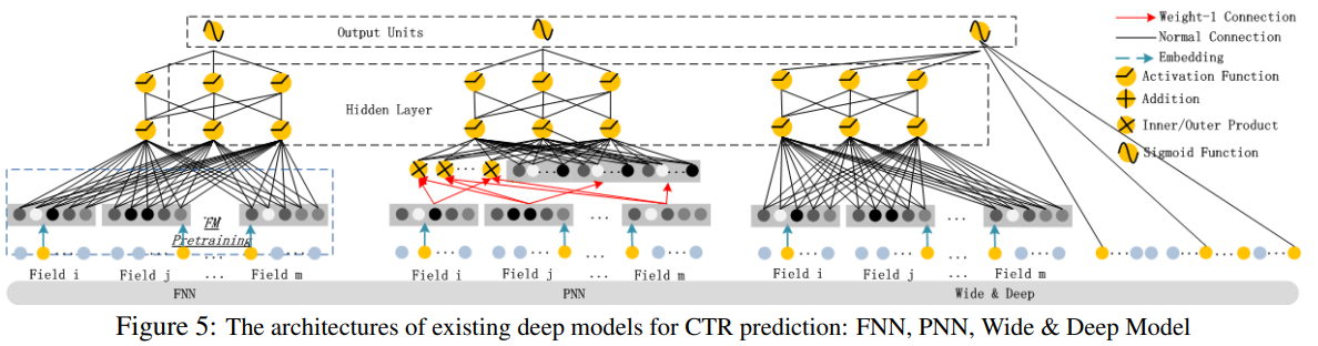
可以看出,现有模型偏向于低阶或高阶特征交互,或者依赖于特征工程。DeepFM 模型能够以端到端的方式学习所有阶的特征交互,除了原始特征外,不需要任何特征工程。与现有模型的比较,如下所示:

2.2 DeepFM 模型的原理
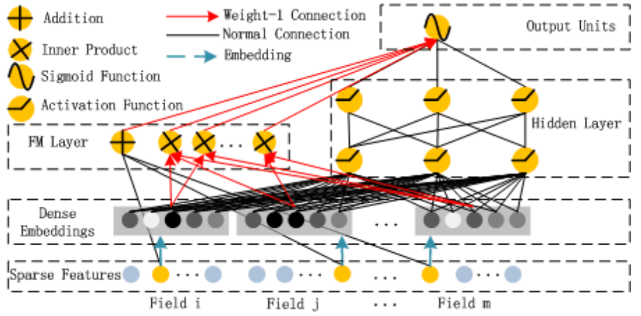
DeepFM 由两个组件组成,即 FM 组件和 deep 组件,它们共享相同的输入。
2.2.1 FM Component

Normal Connection in black refers to a connection with weight to be learned; Weight-1 Connection, red arrow, is a connection with weight 1 by default
它可以比以前的方法更有效地捕获二阶特征交互,尤其是在数据集稀疏的情况下。在以前的方法中,只有当特征 i 和特征 j 都出现在同一数据记录中时,才能训练特征 i 和 j 的交互作用参数。在 FM 中,通过其潜在向量 Vi 和 Vj 的内积进行测量。由于这种灵活的设计,FM可以在i(或j)出现在数据记录中时训练潜在向量Vi(Vj)。因此,FM可以更好地学习从未或很少出现在训练数据中的特征交互。
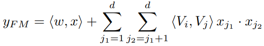
FM 的输出是一个加法单元和若干内积单元的总和:
2.2.2 Deep Component

Deep Module 是为了学习高阶的特征组合,在上图中使用用全连接的方式将 Dense Embedding 输入到 Hidden Layer,这里面 Dense Embeddings 就是为了解决DNN中的参数爆炸问题,这也是推荐模型中常用的处理方法。
2.3 DeepFM 模型的优劣
2.3.1 Efficiency Comparison

纵轴的指标越小,说明效率越高。指标代表的是相对于 LR 模型训练时间的倍数。
2.3.2 Effectiveness Comparison

2.4 Criteo 实战案例
2.4.1 任务和数据介绍
实战使用的数据集是 Criteo 广告数据集,它包含数百万个展示广告的点击反馈记录,该数据可作为点击率(CTR)预测的基准。数据集具有40个特征,第一列是标签,其中值 1 表示已点击广告,而值 0 表示未点击广告。其他特征包含13个dense特征和26个sparse特征。全量csv数据下载:https://cowtransfer.com/s/3f5e873a254b43
任务描述:根据一些特征,可能包括用户的个人属性及其过去行为等,预测某用户是否会点击展示广告。数据中的每一行就是一个独立的样本。
2.4.2 数据载入与预处理
首先,要载入相关的库,并固定随机数种子便于复现
import numpy as np
import pandas as pd
import torch
from torch_rechub.models.ranking import WideDeep, DeepFM, DCN
from torch_rechub.trainers import CTRTrainer
from torch_rechub.basic.features import DenseFeature, SparseFeature
from torch_rechub.utils.data import DataGenerator
from tqdm import tqdm
from sklearn.preprocessing import MinMaxScaler, LabelEncoder
torch.manual_seed(2022) #固定随机种子
data_path = '../examples/ranking/data/criteo/criteo_sample.csv'  # 非全量数据
data = pd.read_csv(data_path)
data.head()
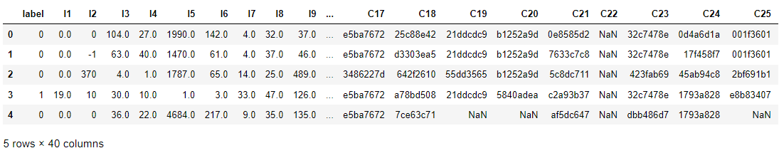
其中以字母 I 为前缀的是 Dense 特征,以字母 C 为前缀的是 Sparse 特征。
2.4.3 特征工程
dense_cols= [f for f in data.columns.tolist() if f[0] == "I"] #以I开头的特征名为dense特征
sparse_cols = [f for f in data.columns.tolist() if f[0] == "C"]  #以C开头的特征名为sparse特征

data[dense_cols] = data[dense_cols].fillna(-996) # 填充空缺值
data[sparse_cols] = data[sparse_cols].fillna('-996')  # 对996的控诉!!!


def convert_numeric_feature(val):  # 某竞赛第一名使用的离散化方法,只知道好用,但尚不清楚原理
    v = int(val)
    if v > 2:
        return int(np.log(v)**2)
    else:
        return v - 2

for col in tqdm(dense_cols):  #将离散化dense特征列设置为新的sparse特征列
    sparse_cols.append(col + "_sparse")
    data[col + "_sparse"] = data[col].apply(lambda x: convert_numeric_feature(x))

scaler = MinMaxScaler()  #对dense特征列归一化
data[dense_cols] = scaler.fit_transform(data[dense_cols])

for col in tqdm(sparse_cols):  #sparse特征编码
    lbe = LabelEncoder()
    data[col] = lbe.fit_transform(data[col])

# 重点:将每个特征定义为torch-rechub所支持的特征基类,dense特征只需指定特征名,sparse特征需指定特征名、特征取值个数(vocab_size)、embedding维度(embed_dim)
dense_features = [DenseFeature(feature_name) for feature_name in dense_cols]
sparse_features = [SparseFeature(feature_name, vocab_size=data[feature_name].nunique(), embed_dim=16) for feature_name in sparse_cols]

# 生成x 和 y
y = data["label"]
del data["label"]
x = data

x
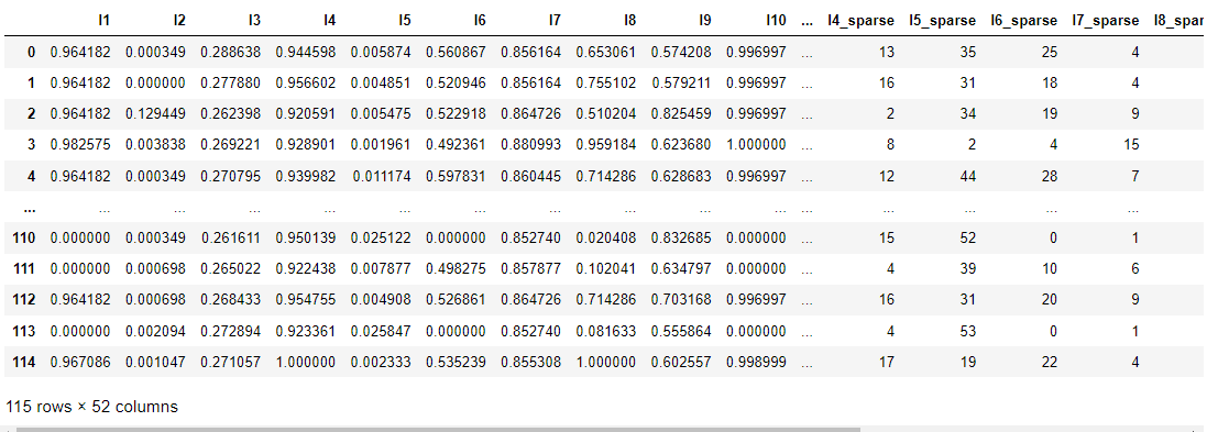
可以看出来,新的数据增加了 12 列,均是 Dense 特征离散化后的结果。
2.4.4 实验设置
# 构建模型输入所需要的dataloader,区分验证集、测试集,指定batch大小
#split_ratio=[0.7,0.1] 指的是训练集占比70%,验证集占比10%,剩下的全部为测试集
dg = DataGenerator(x, y)
train_dataloader, val_dataloader, test_dataloader = dg.generate_dataloader(split_ratio=[0.7, 0.1], batch_size=30, num_workers=4)
# Output: the samples of train : val : test are  80 : 11 : 24
2.4.5 训练和测试
from torch_rechub.models.ranking import DeepFM
from torch_rechub.trainers import CTRTrainer

#定义模型
model = DeepFM(
        deep_features=dense_features+sparse_features,  # FM 和 Deep 模块可以共享输入,不必担心会有冗余的信息
        fm_features=sparse_features,
        mlp_params={"dims": [256, 128], "dropout": 0.2, "activation": "relu"},
    )

# 模型训练,需要学习率、设备等一般的参数,此外我们还支持earlystoping策略,及时发现过拟合
ctr_trainer = CTRTrainer(
    model,
    optimizer_params={"lr": 1e-4, "weight_decay": 1e-5},
    n_epoch=10,
    earlystop_patience=3,
    device='cpu', #如果有gpu,可设置成cuda:0
    model_path='./', #模型存储路径
)
ctr_trainer.fit(train_dataloader, val_dataloader)

# 查看在测试集上的性能
auc = ctr_trainer.evaluate(ctr_trainer.model, test_dataloader)
print(f'test auc: {auc}')

性能不是很好,这可能是因为实验的数据集太小的原因。
2.5 重要源码的解析
class DeepFM(torch.nn.Module):
    """Deep Factorization Machine Model

    Args:
        deep_features (list): the list of `Feature Class`, training by the deep part module.
        fm_features (list): the list of `Feature Class`, training by the fm part module.
        mlp_params (dict): the params of the last MLP module, keys include:`{"dims":list, "activation":str, "dropout":float, "output_layer":bool`}
    """

    def __init__(self, deep_features, fm_features, mlp_params):
        super(DeepFM, self).__init__()
        self.deep_features = deep_features
        self.fm_features = fm_features
        self.deep_dims = sum([fea.embed_dim for fea in deep_features])
        self.fm_dims = sum([fea.embed_dim for fea in fm_features])
        self.linear = LR(self.fm_dims)  # 1-odrder interaction
        self.fm = FM(reduce_sum=True)  # 2-odrder interaction
        self.embedding = EmbeddingLayer(deep_features + fm_features)
        self.mlp = MLP(self.deep_dims, **mlp_params)

    def forward(self, x):
        input_deep = self.embedding(x, self.deep_features, squeeze_dim=True)  #[batch_size, deep_dims]
        input_fm = self.embedding(x, self.fm_features, squeeze_dim=False)  #[batch_size, num_fields, embed_dim]

        y_linear = self.linear(input_fm.flatten(start_dim=1))
        y_fm = self.fm(input_fm)
        y_deep = self.mlp(input_deep)  #[batch_size, 1]
        y = y_linear + y_fm + y_deep
        return torch.sigmoid(y.squeeze(1))

 浙公网安备 33010602011771号