93 Fuzzy Qlearning and Dynamic Fuzzy Qlearning

This part proposes two reinforcement-based learning algorithms. The first, named Fuzzy Q-learning, in an adaptation of Watkins' Q-learning for fuzzy Inference systems. The second, named Dynamical Fuzzy Q-learning, eliminates some drawbacks of both Q-learning and Fuzzy Q-learning. These algorithms are used to improve the rule based of a fuzzy controller.

Introduction##

In the reinforcement learning paradigm, an agent receives from its environment a scalar reward value called \(reinforcement\). This feedabck is rather poor: it can be loolean (true, false) or fuzzy (bad, fair, very good...), and, moreover, it may be delayed. A sequence of control actions is often executed before receiving any information on the quality of the whole sequence. Therefore, it is difficult to evaluate the contribution of one individual action.

This \(Credit Assignment Problem\) has been widely studied since the pioneering work of Barto, Sutton and Anderson. The whole methodology is called Temporal Difference Method and contains a family of algorithms. Recently, Watkins proposed a new algorithm of this family, Q-learning.

Q-learning##

Q-learning is a form of competive learning which provides agents with the capability of learning to act optimally by evaluating the consequences of actions. Q-learning keeps a Q-function which attempts to estimate the discounted future reinforcement for taking actions from given states. A Q-function is a mapping from state-action pairs to predicted reinforcement. In order to explain the method, we adopt the implementation proposed by Bersini.

1. The state space, \(U\subset R^{n}\), is partitioned into hypercubes or cells. Among these cells we can distinguish:

   a. one particular cell, called the target cell, to which the quality value +1 is assigned,

   b. a subset of cells, called viability zone, that the process must not leave. The quality value for viability zone is 0. This notion of viability zone comes from Aubin and eliminates strong constraints on a reference trajectory for the process.

   c. the remaining cells, called failure zone, with the quality value -1.

2. In each cell, a set of \(J\) agents compete to control a process. With \(M\) cells, the agent \(j\), \(j\in \{ 1,\ldots,J \}\), acting in cell \(c\), \(c\in \{ 1,\ldots, M \}\), is characterized by its quality value \(Q[c,j]\). The probability to agent \(j\) in cell \(c\) will be selected is given by a Boltzmann distribution.

3. The selected agent controls the process as long as the process stays in the cell. When the process leaves cell \(c\) to get into cell \(c^{'}\), at time step \(t\), another agent is selected for cell \(c^{'}\) and the Q-function of the previous agent is incremented by:

\[\Delta Q[c,j] = \alpha\{ r(t)+ \gamma \underset{k}{\max} Q[k,c^{'}]-Q[c,j] \} \]

where \(\alpha\) is the learning rate (\(\alpha<1\)), \(\gamma\) the discount rate \((\gamma<1)\) and \(r(t)\) the reinforcement.

\[r(t)=\left\{\begin{matrix} +1 & {\rm if} \ c^{'}\ {\rm is \ the \ target \ cell \ (reward)}\\ 0& {\rm if} \ c^{'}\ {\rm is \ in\ the \ viability \ zone } \\ -1& {\rm if} \ c^{'}\ {\rm is \ in \ the \ failure \ zone \ (punishment)} \end{matrix}\right.\]

It is shown in the following equation that \(Q[c,j]\) tends towards the discounted cumulative reward \(R_{t}\):

\[R_{t}=\sum_{n=0}^{\infty}\gamma^{n}r_{t+n}$$. This method is very attractive because it performs an on-line medol-free optimization of a control policy, enabling the identification of the best operator at any time. But, infortunately, Q-learning is slow and serval authors have proposed extension inorder to reduce the problem search space so as to accelerate learning. For example, Lin[10] proposes experence replay and teaching. Whitechead [16] adds a biasing function to the Q-function, with an external teacher providing shorter latence feedback. Clouse and Utgloff [11] uses transitional proximity: the states closest to the current state receive correspondingly more of the current reward. ##Fuzzy Inference Systems## We consider a FIS with $N$ fuzzy rules on the form: $${\rm rule} \ \bm{i}:{\rm \bm{if}}\ x_{1}\ is \ A_{1}^{i(1)} \ {\rm and } \ x_{2} \ is \ {\rm A_{2}^{i(2)}} \ldots \ {\rm and } \ x_{n} \ {\rm is} \ A_{n}^{i(n)} \ {\rm then } y \ {\rm is} \ B^{i} \]

where \((A_{j}^{i(j)})_{j=1,n}\) and \(B^{i}\), \(i=1, \ldots, N\), are fuzzy subsets characterized by linguistic lables (e.g. "small", "medium", "positive large", ...) and by a function \(x \rightarrow \mu _{A}(x)\in[0,1]\), called membership function, quantifying the membership degree of \(x\) to \(A\).

This FIS is charaterized by:

1. Any parametrable input membership function. The function parameters must allow dilatation and translation. We suppose that the output membership functions have one point, \(b^{i}\), such that \(\mu_{B^{i}}(b^{i}) =1\).
2. Any conjunction operator (generalization of the boolean \(And\)), e.g. Minimum, product or Lukasiewicz conjunction.
3. Product inference.
4. Centroid defuzzification.

For an input vector, \(\bm{x}\), the inferred output, \(y\), is:

\[y=\frac{ \sum_{i=1}^{N} \alpha_{i} (\bm{x} ) \times b^{i} }{ \sum_{j=1}^{N} \alpha_{j}( \bm{x} ) }$$, where $\alpha_{i} (\bm{x} )$ is the stength of rule $i$. It is shown in [8] that such FIS are universal approximatros and that they can learn by exmaples. The most important features of FIS are that thay can imcorporate human prior knowledge into their parameters and that these parameters have clear physical meaning. Tuning a FIS consists in going from qualitative to qualitative: how can parameters be tuned so that a FIS performs a desired nonlinear mapping? In the following, we show that an adaptation of Q-learning enables the best rule among a set of possible rule bases to be found. ##Fuzzy Q-Learning## Fuzzy Q-learning is an immediate extension of the basic method. For simplicity we take a fuzzy partition of each input variable domain, for example with triangles crossing at grade 0.5. Therefore, for an input vertor, $x\in R^{n}$, only $2^{n}$ rules are fired. The set is defined by: $$H_{j(1),\ldots,j(2^{n})}=\{ \bm{x} \in R^{n} | \alpha_{j(1)}(\bm{x})\neq 0,\ldots, \alpha_{j(2^{n})}(\bm{x})\neq 0 \}\]

is a hypercube in \(R^{n}\), \(j(i)\in \{ 1,\ldots,N \}\) for \(i=1,\ldots,2^{n}\), \(j(i) \neq j(k)\) if \(i \neq k\). In the vertices of these hypercubes, only one rule is fired, with truth value 1.

These bypercubes form a partition of the state space into cells which are divided into a target cell, a hypercubes, a viability zone and a failure zone.

We define \(J\) sets of fuzzy rules sharing the same antecedent parts. In our implementation, an agent is equivalent to a fuzzy rule base, it acts on the whole state space but computes its control action for each hypercube (cell). Rule number \(i\), \(i=1,\ldots, N\), of agent number \(j\), \(j=1, \ldots, J\), is now:

\[{\rm rule} \ \bm{i}:{\rm \bm{if}}\ x_{1}\ is \ A_{1}^{i(1)} \ {\rm and } \ x_{2} \ is \ {\rm A_{2}^{i(2)}} \ldots \ {\rm and } \ x_{n} \ {\rm is} \ A_{n}^{i(n)} \ {\rm then } \ y \ {\rm is} \ B^{i} (j) \]

The set of agents is implemented by a FIS with \(J\) outputs, see

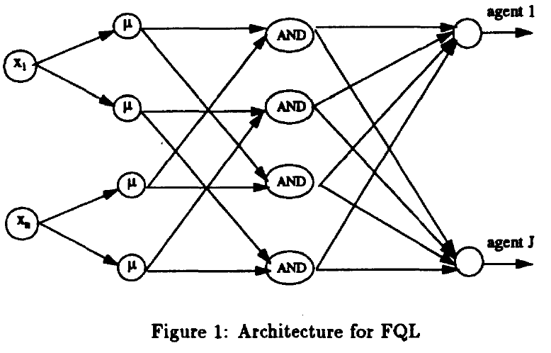
For each agent, we define:

1. A Q-function, \(Q[c,j]\), where \(c\) refers to the cell and \(j\) the agent.
2. A rule quality, \(q[k,j]\), for rule number \(k\) used by agent number \(j\).

The relation between \(Q\) and q-function is given by:

\[Q[c,j] = \frac{1}{2^{n}} \sum_{k\in H(c)} q[k,j] \]

where \(H(c)\) refers to the fired rules when the input vector is in cell number \(c\). \(Q[c,j]\) is the mean value of \(q[k,j]\) for \(k\in H(c)\).

If \(j_{0}\) is the number of the active agent, its Q-function, \(Q[c,j_{0}]\), is updated by