【吴恩达】引言、线性回归、多项式回归

Machine Learning

Chapter1 Introduction

What is machine learning

A computer program is said to learn from experience E with respect to some task T and some performance measure P, if its performance on T, as measured by P, improves with experience E.

某类任务T（task）具有性能度量P（performance），计算机程序可以从任务T的经验E（experience）中学习，提高性能P.

Machine learning algorithms can be divided into Supervised learning and Unsupervised learning.

Supervised learning

Given the label

• Classification: Discrete valued output
• regression: Continuous valued output

Unsupervised learning

Not given the label

• cluster
• cocktail party

Chapter2 Univariate Linear Regression

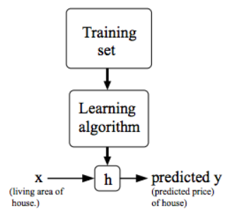
Model representation

Hypothesis function

\[h_\theta(x) = \theta_0+\theta_1 x \]

hypothesis: just a terminology. Here we assume the initial expression of the model is linear(easiest, can also be quadratic or multiple order).

Cost function

Square error function: The most commanly used one for regression problems.

\[J(\theta_0,\theta_1)=\frac{1}{2m} \sum_1^m[h_\theta(x^{(i)})-y^{(i)}]^2 \]

m means the number of data sets, i.e. the number of points in the image.

Adding \(\frac{1}{2}\) only to get a easier function after derivation, which has no effect to the optimization results.

Goal: Choose \(\theta_0,\theta_1\) so that \(J(\theta_0,\theta_1)\) is minimum

\[\min_{\theta_0,\theta_1}J(\theta_0,\theta_1) \]

Each value group of \((\theta_0,\theta_1)\) corresponds to a different hypothesis function, and a different cost value.

\(J\) is a function with respect to \(\theta\), \(h_\theta\) is a function with respect to \(x\), the number of \(\theta\) is always more than the number of \(x\), so \(J\) always has a higher dimension than \(h_\theta\).

We use hypothesis function and original value to get cost function. Then, find the minimum cost value in cost function, so that we find the most suitable Hypothesis function to fit the original data.

Gradient descent

repeat until convergence{

for \(j=0\) and \(j=1\)

\[\theta_j=\theta_j-\alpha\frac{\partial}{\partial\theta_j}J(\theta_0,\theta_1) \]

\(\alpha\) is called learning rate. If \(\alpha\) is too small, gradient descent can be slow; If \(\alpha\) is too large, gradient descent can overshoot the minimum, which may fail to converge, or even diverge.

}

note: simultaneous update. We need two temporary variables to implement this.

Cost function for linear regression is always going to be a convex function. So we needn't worry about the local optima question.

Batch Gradient Descent: each step of gradient descent uses all the training examples.

Multivariate Linear Regression

Hypothesis function

\[\begin{aligned} h_\theta(x) &= \theta_0x_0+\theta_1x_1+\theta_2x_2+\cdots+\theta_nx_n \\&=\theta^Tx \end{aligned} \\ \theta= \left[ \begin{matrix} \theta_0\\ \theta_1\\ \vdots\\ \theta_n \end{matrix} \right] ,x= \left[ \begin{matrix} x_0\\ x_1\\ \vdots\\ x_n \end{matrix} \right] (x_0=1) \]

n means the number of features,i.e. the number of axis in the image. In univariate linear regression, n=1.

Cost function

\[J(\theta)=\frac{1}{2m} \sum_1^m[h_\theta(x^{(i)})-y^{(i)}]^2 \]

Unlike univariate linear regression, here \(\theta\) and \(x\) are both vectors rather than scalers.

Gradient descent

repeat until convergence{

\[\begin{aligned} \theta_j&=\theta_j-\alpha\frac{\partial}{\partial\theta_j}J(\theta)\\ &=\theta_j-\frac{\alpha}{m} \sum_1^m[h_\theta(x^{(i)})-y^{(i)}]x_j^{(i)} \end{aligned} \]

(simultaneously update for every \(j=0,\cdots,n\))

}

In order to make gradient descent run much faster and converge in a lot fewer iterations, here are some tricks.

Feature scaling

If the value of one feature is far larger than the other feature, then the contour of the cost function will be a bunch of skinny ovals, the gradient descent will be very slow.

Get every feature into approximately a \(-1\le x_i\le1\) range.

Mean normalization

Replace \(x_i\) with \(x_i-\mu_i\) to make features have approximately zero mean. Do not apply to \(x_0\), because \(x_0 \equiv 1\), no matter how we transform.

Learning rate

Plot the figure of cost function with respect to the number of iterations, in order to check the convergence.

• If the curve is increasing or oscillating, use smaller \(\alpha\)
• If the curve decreases too slowly, use larger \(\alpha\)

Normal equation

m examples, n features.

\[x^{(i)}= \left[ \begin{matrix} x_0^{(i)}\\ x_1^{(i)}\\ x_2^{(i)}\\ \vdots\\ x_n^{(i)}\\ \end{matrix} \right]_{(n+1)\times1} , X= \left[ \begin{matrix} (x^{(1)})^T\\ (x^{(2)})^T\\ (x^{(3)})^T\\ \vdots\\ (x^{(m)})^T\\ \end{matrix} \right]_{m\times(n+1)} , y^{(i)}= \left[ \begin{matrix} y^{(1)}\\ y^{(2)}\\ y^{(3)}\\ \vdots\\ y^{(m)}\\ \end{matrix} \right]_{m\times1} \]

\[\theta=(X^TX)^{-1}X^Ty \]

No need to do feature scaling.

what if \(X^TX\) is non-invertible(singular or degenerate), although we run this pretty rarely?

• Redundant features(linearly dependent). We should delete the redundant features
• Too many features(\(m\le n\)).We should delete some features, or use regularization.

Gradient descent vs Normal equation

Gradient descent

• Need to choose \(\alpha\). This means running it few times with different \(\alpha\) and seeing which works best.
• Need many iterations. This may very slow in some cases(ellipse), and need to plot J of No. iterations to check the convergence.
• Work well even when \(n\) is large.

Normal equation

• No need to choose \(\alpha\)
• No need to iterate.
• Slow when \(n\) is large(\(n>10000\)). Need to compute \((X^TX)^{-1}\), which is an (n+1)\(\times\)(n+1) matrix. Compute matrix with large dimensions takes much time, the time complexity is \(o(n^3)\).

Chapter3 Polynomial regression

Hypothesis Function

\[\begin{aligned} h_\theta(x) &= \theta_0+\theta_1x+\theta_2x^2+\theta_3x^3 \\&= \theta_0+\theta_1x_1+\theta_2x_2+\theta_3x_3 \end{aligned} \]

\[x_1=x,x_2=x^2,x_3=x^3 \]

Transform the polynomial function to multivariate function. Remember to use feature scaling.

words and expressions

pseudo 伪

resort 求助

sophisticated 复杂的

quadratic 二次 cubic 三次

skinny 瘦的

ellipse oval 椭圆

skewed 歪曲的

malignant tumor 恶性肿瘤

benign tumor 良性肿瘤

lump 肿块

tragical 悲剧性的

slightly 轻微地

clump 簇、群

inventory 库存清单

cohesive 有结合力的

diabetes 糖尿病

hypothesis 假设

intuition 直觉

contour 等高线

colon 冒号

comma 逗号

whereas 鉴于、然而

susceptible 易受影响的

iterative 迭代的

commutative property 交换律

associative property 结合律

sloppy 马虎的，草率的