PCA主成分分析
PCA主成分分析
是一种降维算法
"""
# @Time : 2020/8/21
# @Author : Jimou Chen
"""
from sklearn.neural_network import MLPClassifier # 待会用神经网络预测降维后的数据
from sklearn.datasets import load_digits # 手写数据集
from sklearn.model_selection import train_test_split
from sklearn.decomposition import PCA # 导入PCA模型
from sklearn.metrics import classification_report, confusion_matrix
import matplotlib.pyplot as plt
# from mpl_toolkits.mplot3d import Axes3D
digits = load_digits()
x_data = digits.data # 数据
y_data = digits.target # 标签
# 切分数据
x_train, x_test, y_train, y_text = train_test_split(x_data, y_data)
# 建立神经网络模型,包含两个隐藏层,分别有100和50个神经元
model = MLPClassifier(hidden_layer_sizes=(100, 50), max_iter=500)
model.fit(x_train, y_train)
# 评估
prediction = model.predict(x_test)
print(prediction)
print(classification_report(prediction, y_text))
print(confusion_matrix(prediction, y_text))
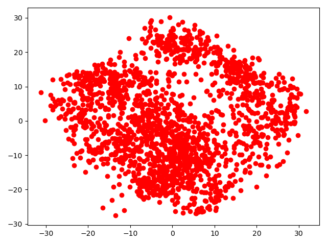
# 进行pca降维,这里n_components是降成2维
pca = PCA(n_components=2)
# 直接返回降维后的数据,如果不返回新数据,就用fit
new_data = pca.fit_transform(x_data)
print(new_data)
# 画出降维后的数据
new_x_data = new_data[:, 0]
new_y_data = new_data[:, 1]
plt.scatter(new_x_data, new_y_data, c='r')
plt.show()
# 这里的是只拟合,不返回重构的新数据
pca = model.fit(x_train, y_train)
pred = model.predict(x_data)
print(classification_report(pred, y_data))
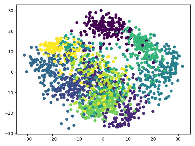
# 画出预测的聚类图
plt.scatter(new_x_data, new_y_data, c=pred)
# plt.scatter(new_x_data, new_y_data, c=y_data)
plt.show()
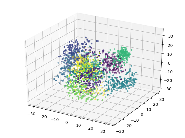
'''降成3个维度'''
pca = PCA(n_components=3)
new_data = pca.fit_transform(x_data)
# 画出降维后的数据
new_x_data = new_data[:, 0]
new_y_data = new_data[:, 1]
new_z_data = new_data[:, 2]
ax = plt.figure().add_subplot(111, projection='3d')
ax.scatter(new_x_data, new_y_data, new_z_data, c=pred, s=10)
# ax.scatter(new_x_data, new_y_data, new_z_data, c=y_data, s=10)
plt.show()
-
运行结果
-
输出结果
[4 8 4 9 7 8 5 7 0 4 4 2 6 3 6 4 5 8 4 1 8 7 4 5 4 5 7 6 4 4 5 1 5 7 0 1 5
 3 4 8 3 5 4 6 3 9 3 8 0 1 7 3 4 5 4 8 0 4 2 8 9 6 7 9 4 6 2 5 7 5 8 6 0 0
 8 8 3 0 6 7 6 8 5 0 0 9 4 8 4 3 9 8 9 8 4 0 7 2 0 3 8 5 4 2 6 5 9 2 0 6 3
 8 1 1 7 5 4 3 4 6 7 5 8 7 5 1 8 1 8 4 2 7 4 2 5 8 9 8 9 2 5 5 9 6 1 7 7 6
 7 0 4 4 9 3 2 4 4 3 3 3 6 5 5 4 4 4 0 3 1 7 6 9 2 9 8 5 9 8 8 9 4 0 9 3 3
 6 4 1 8 5 9 6 6 5 8 0 8 1 2 9 8 1 5 5 0 1 3 7 2 7 9 0 3 0 1 8 7 5 9 5 1 9
 3 6 5 1 1 8 7 7 2 0 7 3 7 1 1 7 4 4 1 9 9 3 2 0 8 2 4 7 9 2 5 3 4 5 1 0 4
 3 0 6 5 0 7 4 3 6 5 9 9 6 1 6 9 9 5 1 4 5 3 5 8 0 1 0 8 5 3 0 2 6 6 2 9 3
 7 3 0 0 4 3 3 2 4 7 6 8 5 5 9 2 9 0 7 2 0 9 8 2 3 6 5 1 8 7 5 2 1 0 9 3 6
 4 2 8 4 1 3 0 2 9 6 5 1 2 1 1 8 5 1 4 2 3 5 3 3 7 0 8 0 8 6 5 8 7 6 2 8 8
 1 4 3 5 8 5 5 6 9 9 5 8 4 9 7 2 9 6 3 6 5 7 5 9 8 9 6 9 0 0 4 4 4 1 6 4 3
 2 9 5 1 2 9 2 5 8 5 2 4 2 0 3 1 0 4 5 8 4 5 6 5 1 2 6 2 5 7 0 3 3 6 7 3 7
 8 2 3 8 4 8]
              precision    recall  f1-score   support

           0       1.00      1.00      1.00        40
           1       0.97      1.00      0.99        37
           2       0.97      0.97      0.97        38
           3       0.98      0.93      0.96        46
           4       1.00      0.96      0.98        55
           5       0.97      0.95      0.96        59
           6       1.00      1.00      1.00        40
           7       0.97      1.00      0.99        39
           8       0.93      1.00      0.96        52
           9       1.00      0.98      0.99        44

    accuracy                           0.98       450
   macro avg       0.98      0.98      0.98       450
weighted avg       0.98      0.98      0.98       450

[[40  0  0  0  0  0  0  0  0  0]
 [ 0 37  0  0  0  0  0  0  0  0]
 [ 0  0 37  0  0  0  0  0  1  0]
 [ 0  1  1 43  0  1  0  0  0  0]
 [ 0  0  0  0 53  1  0  0  1  0]
 [ 0  0  0  1  0 56  0  0  2  0]
 [ 0  0  0  0  0  0 40  0  0  0]
 [ 0  0  0  0  0  0  0 39  0  0]
 [ 0  0  0  0  0  0  0  0 52  0]
 [ 0  0  0  0  0  0  0  1  0 43]]
[[ -1.25946953  21.2748899 ]
 [  7.95760889 -20.76869375]
 [  6.99192912  -9.95599846]
 ...
 [ 10.80128058  -6.9602433 ]
 [ -4.87210255  12.42397333]
 [ -0.34439116   6.36555361]]
              precision    recall  f1-score   support

           0       1.00      1.00      1.00       178
           1       0.99      0.99      0.99       183
           2       1.00      0.99      1.00       178
           3       0.99      0.99      0.99       182
           4       0.99      0.99      0.99       182
           5       0.99      0.98      0.99       183
           6       1.00      1.00      1.00       181
           7       0.99      1.00      1.00       178
           8       0.97      0.98      0.98       172
           9       0.99      0.99      0.99       180

    accuracy                           0.99      1797
   macro avg       0.99      0.99      0.99      1797
weighted avg       0.99      0.99      0.99      1797


Process finished with exit code 0

 浙公网安备 33010602011771号