灰度变换之分段变换
 基于Python详解伽马变换在数字图像处理的作用
1. 概述
数字图像处理中分段变换就是对不同的灰度区间应用不同的变换函数,从而可以增强感兴趣的灰度区间、抑制不感兴趣的灰度级
分段线性函数的优点是可以根据需要拉伸特征物的灰度细节,一些重要的变换只能用分段函数来描述和实现,缺点则是参数较多不容易确定
分段线性函数典型图像如下:
In [1]:
import numpy as np
import matplotlib.pyplot as plt

def func(value):
    if value <= 3:
        return 0
    if value <= 6:
        return 2*(value-3)
    else:
        return 6
plt.figure(figsize=(6,4))
x = np.linspace(0, 8, 100)
y = np.array([])
for v in x:
    y = np.append(y,np.linspace(func(v),func(v),1))
l=plt.plot(x,y,'b',label='value')
plt.text(3.2, 0.2, r'$x_1,y_1$')
plt.text(6, 5.7, r'$x_2,y_2$')
plt.legend()
plt.show()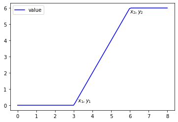
分段线性函数通用公式如下:
$$ f(x) = \left\{ \begin{matrix} \frac {y_1}{x_1}x \ \ \ \ \ \ \ \ \ \ \ ,\ x<x_1\\ \frac {y_2-y_1}{x_2-x_1}x+y_1 \ \ \ \ \ \ \ \ , \ x_1<x<x_2 \\ \frac {y_{max} \ \ - y_2}{x_{max}\ \ -x_2}x + y_2 \ \ \ , \ x>x_2 \\ \end{matrix} \right. $$
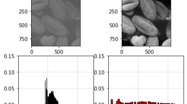
利用分段变换,可以将图像某一区间的灰度值扩大,从而将灰度值集中在某一区间的图像对比度增强
2. 伽马变换的弊端
非分段变换(如,伽马变换)会存在一个斜率大约为1的区间,这使得在这个区间的图像进行伽马变化后对比度几乎无变化
In [2]:
from PIL import Image
import numpy as np
import matplotlib.pyplot as plt

def gamma_trans(input, gamma=2, eps=0 ):
    return 255. * (((input + eps)/255.) ** gamma)

# 读入原图
gray_img = np.asarray(Image.open('./image/washed_out_pollen_image.tif').convert('L'))

# 创建一个显示主体,并分成四个显示区域
fig = plt.figure()
ax1 = fig.add_subplot(221)
ax2 = fig.add_subplot(222)
ax3 = fig.add_subplot(223)
ax4 = fig.add_subplot(224)

# 显示原图
ax1.set_title("origin")
ax1.imshow(gray_img, cmap='gray', vmin=0, vmax=255)
ax1.axes.xaxis.set_visible(False)
ax1.axes.yaxis.set_visible(False)

# 显示原图的灰度分布直方图
ax2.grid(True, linestyle=':', linewidth=1)
ax2.set_title('origin', fontsize=12)
ax2.set_xlim(0, 255)  # 设置x轴分布范围
ax2.set_ylim(0, 0.15)  # 设置y轴分布范围
ax2.hist(gray_img.flatten(), bins=50,density=True,color='r',edgecolor='k')
ax2.axes.xaxis.set_visible(False)
ax2.axes.yaxis.set_visible(False)

gamma_ = 2
# 对原图执行γ变换
output = gamma_trans(gray_img, gamma_, 0.2)

# 显示γ变换结果图像
ax3.set_title("result")
ax3.imshow(output, cmap='gray',vmin=0,vmax=255)
ax3.axes.xaxis.set_visible(False)
ax3.axes.yaxis.set_visible(False)

# 显示γ变换结果图像的灰度分布直方图
ax4.set_xlim(0, 255)  # 设置x轴分布范围
ax4.set_ylim(0, 0.15)  # 设置y轴分布范围
ax4.grid(True, linestyle=':', linewidth=1)
ax4.set_title('result', fontsize=12)
ax4.hist(output.flatten(),bins=50,density=True,color='r',edgecolor='k')
ax4.axes.xaxis.set_visible(False)
ax4.axes.yaxis.set_visible(False)

plt.show()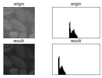
可以看到,对于灰度值集中于中间某一个部分的图像,伽马变化几乎无法提升对比度
3. 分段变换
根据分段函数公式:
$$ f(x) = \left\{ \begin{matrix} \frac {y_1}{x_1}x \ \ \ \ \ \ \ \ \ \ \ ,\ x<x_1\\ \frac {y_2-y_1}{x_2-x_1}x+y_1 \ \ \ \ \ \ \ \ , \ x_1<x<x_2 \\ \frac {y_{max} \ \ - y_2}{x_{max}\ \ -x_2}x + y_2 \ \ \ , \ x>x_2 \\ \end{matrix} \right. $$
我们可以写出最简单直接的分段变换函数:
In [3]:
# 三段对比度拉伸变换,其中x1,y1和x2,y2为分段点,x是输入矩阵
def three_linear_trans(x, x1,y1, x2,y2):
    # 1.检查参数,避免分母为0
    if x1 == x2 or x2 == 255:
        print("[INFO] x1=%d,x2=%d ->调用此函数必须满足:x1≠x2且x2≠255" % (x1, x2))
        return None

    # 2.执行分段线性变换
    out = np.zeros(x.shape)
    for i in range(x.shape[0]):
        for j in range(x.shape[1]):
            if x[i,j] < x1:
                out[i,j] = y1/x1*x[i,j]
            elif x1 <= x[i,j] <= x2:
                out[i,j] = (y2-y1)/(x2-x1)*(x[i,j]-x1)+y1
            elif x[i,j] > x2:
                out[i,j] = (255-y2)/(255-x2)*(x[i,j]-x2)+y2
    return out
对刚才的图像进行分段变换:
In [4]:
# 以灰度方式读入图像
gray_img = np.asarray(Image.open('./image/washed_out_pollen_image.tif').convert('L'))

# 创建一个显示主体,并分成五个显示区域
fig = plt.figure()
ax1 = fig.add_subplot(221)
ax2 = fig.add_subplot(222)
ax3 = fig.add_subplot(223)
ax4 = fig.add_subplot(224)

# 显示原图及其灰度分布直方图
ax1.set_title("origin", fontsize=8)
ax1.imshow(gray_img,cmap='gray',vmin=0,vmax=255)

ax3.grid(True, linestyle=':', linewidth=1)
ax3.set_xlim(0, 255)  # 设置x轴分布范围
ax3.set_ylim(0, 0.15)  # 设置y轴分布范围
ax3.hist(gray_img.flatten(), bins=50, density=True, color='r', edgecolor='k')

# 执行分段线性变换
x1,y1,x2,y2 = 90, 3, 140, 250
out = three_linear_trans(gray_img,x1,y1,x2,y2)

# 显示变换结果图像
ax2.clear()
ax2.set_title("result", fontsize=8)
ax2.imshow(out,cmap='gray',vmin=0,vmax=255)

# 显示变换结果的灰度分布直方图
ax4.clear()
ax4.grid(True, linestyle=':', linewidth=1)
ax4.set_xlim(0, 255)  # 设置x轴分布范围
ax4.set_ylim(0, 0.15)  # 设置y轴分布范围
ax4.hist(out.flatten(), bins=50, density=True, color='r', edgecolor='k')

plt.show()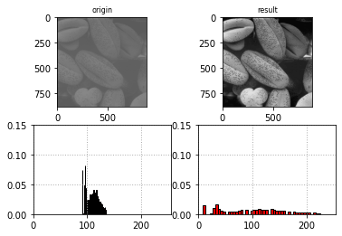
可以看到对比度得到显著增强,颜色分布不再是集中于中间的某个区间
当然,这种把集中于某个区间的颜色进行扩大分布也叫直方图均衡化 (Histogram Equalization) ,指的是对图像的颜色值进行重新分配,使得颜色值的分布更加均匀
4. 算法优化
这里我们充分利用Numpy的广播机制与并行计算,对刚才的分段变换进行优化
通过三个掩码矩阵来实现每一段函数的计算,最后把它们加起来,就是最后的变换结果:
In [5]:
# 三段对比度拉伸变换,其中x1,y1和x2,y2为分段点,x是输入矩阵
def three_linear_trans2(x, x1,y1, x2,y2):
    # 1.检查参数,避免分母为0
    if x1 == x2 or x2 == 255:
        print("[INFO] x1=%d,x2=%d ->调用此函数必须满足:x1≠x2且x2≠255" % (x1, x2))
        return None

    # 2.执行分段线性变换
    out = np.zeros(x.shape)
    m1=(x<x1)
    m2=(x1<=x)&(x<=x2)
    m3=(x>x2)

    out = (y1/x1*x)*m1 + ((y2-y1)/(x2-x1)*(x-x1)+y1)*m2 + ((255-y2)/(255-x2)*(x-x2)+y2)*m3
    return out
执行时间对比:
In [6]:
import time

gray_img = np.asarray(Image.open('./image/washed_out_pollen_image.tif').convert('L'))

x1,y1,x2,y2 = 90, 3, 140, 250

ticks1 = time.time()
out = three_linear_trans(gray_img,x1,y1,x2,y2)
print("消耗时间(s)为:", time.time()-ticks1)

ticks2 = time.time()
out = three_linear_trans2(gray_img,x1,y1,x2,y2)
print("消耗时间(s)为:",  time.time()-ticks2)
消耗时间(s)为: 7.202014446258545
消耗时间(s)为: 0.017905712127685547可以看到执行效率显著提升