时空序列预测1--ConvLSTM原理及keras实现

论文翻译：https://blog.csdn.net/u014386899/article/details/100560734

1 背景

用于降水预测

2 核心思想

2.1 卷积替代hadamard乘积

普通的LSTM是这样的

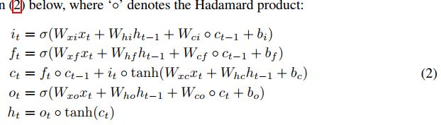
其中的 o 表示hadamard乘积，其实就是矩阵相乘，相当于全连接神经网络（一层全连接网络就是相当于一个矩阵相乘），全连接网络参数量巨大，不能有效提取空间信息，把它换为卷积之后则能有效提取空间信息(花书中使用卷积层替代全连接层的动机)，于是把hadamard乘积改为卷积。
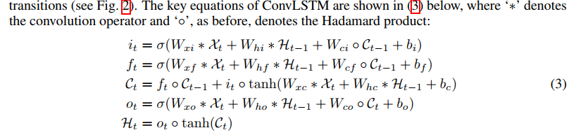
于是就有了ConvLSTM

再来两幅图片来形象的表示一下
LSTM结构图如下：

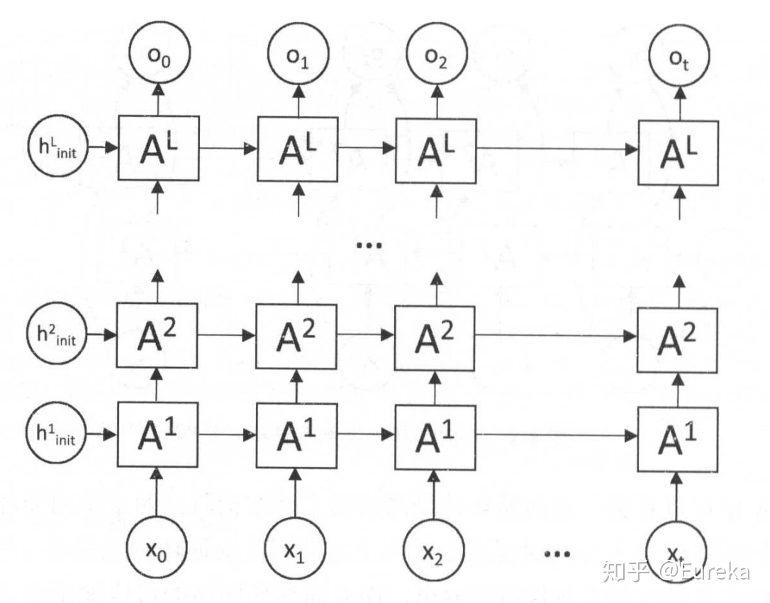
ConvLSTM的结构图如下：

区别也就是一个输入的是一维序列，另一个是二维图片；处理一维序列使用的是卷积全连接神经网络，处理二维图片使用的是卷积神经网络。

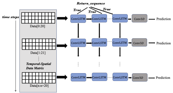
2.2 Encoding-Forecasting结构

这个Encoding-Forecasting结构，其实就相当于使用一个Encoding-Decoding结构(经典论文Sequence to sequence learning with neural networks)，这种结构的目的都是为了实现端到端的直接预测，实现输入是序列，输出也是序列的效果，比如语义分割、自然语言处理中的翻译等，都是用的这样的结构。
在这篇论文中使用这样的结构，可以实现输入是图片，输出也是图片的效果。

3 实现

这是keras的官方代码，下载数据集的时候比较慢，可以把该数据集单独下载之后，再进行训练，对显卡要求比较高，使用1080Ti，把batchsize设置为1勉强跑得动，3090能够跑得动

点击查看代码

'''https://keras.io/examples/vision/conv_lstm/'''
import numpy as np
import matplotlib.pyplot as plt

import tensorflow as tf
from tensorflow import keras
from tensorflow.keras import layers

import io
import imageio
from IPython.display import Image, display
from ipywidgets import widgets, Layout, HBox

#选择指定显卡及自动调用显存
physical_devices = tf.config.experimental.list_physical_devices('GPU')#列出所有可见显卡
print("All the available GPUs:\n",physical_devices)
if physical_devices:
    gpu=physical_devices[0]#显示第一块显卡
    tf.config.experimental.set_memory_growth(gpu, True)#根据需要自动增长显存
    tf.config.experimental.set_visible_devices(gpu, 'GPU')#只选择第一块


#载入数据
# Download and load the dataset.
fpath = keras.utils.get_file(
    "moving_mnist.npy",
    "http://www.cs.toronto.edu/~nitish/unsupervised_video/mnist_test_seq.npy",
)
dataset = np.load(fpath)

# Swap the axes representing the number of frames and number of data samples.
dataset = np.swapaxes(dataset, 0, 1)
# We'll pick out 1000 of the 10000 total examples and use those.
dataset = dataset[:1000, ...]
# Add a channel dimension since the images are grayscale.
dataset = np.expand_dims(dataset, axis=-1)

# Split into train and validation sets using indexing to optimize memory.
indexes = np.arange(dataset.shape[0])
np.random.shuffle(indexes)
train_index = indexes[: int(0.9 * dataset.shape[0])]
val_index = indexes[int(0.9 * dataset.shape[0]) :]
train_dataset = dataset[train_index]
val_dataset = dataset[val_index]

# Normalize the data to the 0-1 range.
train_dataset = train_dataset / 255
val_dataset = val_dataset / 255

# We'll define a helper function to shift the frames, where
# `x` is frames 0 to n - 1, and `y` is frames 1 to n.
def create_shifted_frames(data):
    x = data[:, 0 : data.shape[1] - 1, :, :]
    y = data[:, 1 : data.shape[1], :, :]
    return x, y


# Apply the processing function to the datasets.
x_train, y_train = create_shifted_frames(train_dataset)
x_val, y_val = create_shifted_frames(val_dataset)

# Inspect the dataset.
print("Training Dataset Shapes: " + str(x_train.shape) + ", " + str(y_train.shape))
print("Validation Dataset Shapes: " + str(x_val.shape) + ", " + str(y_val.shape))

#数据可视化
# Construct a figure on which we will visualize the images.
fig, axes = plt.subplots(4, 5, figsize=(10, 8))

# Plot each of the sequential images for one random data example.
#这种显示子图的方法好高级，学习一下
data_choice = np.random.choice(range(len(train_dataset)), size=1)[0]
for idx, ax in enumerate(axes.flat):
    ax.imshow(np.squeeze(train_dataset[data_choice][idx]), cmap="gray")
    ax.set_title(f"Frame {idx + 1}")
    ax.axis("off")

# Print information and display the figure.
print(f"Displaying frames for example {data_choice}.")
plt.show()

#模型构建
# Construct the input layer with no definite frame size.
inp = layers.Input(shape=(None, *x_train.shape[2:]))

# We will construct 3 `ConvLSTM2D` layers with batch normalization,
# followed by a `Conv3D` layer for the spatiotemporal outputs.
x = layers.ConvLSTM2D(
    filters=64,
    kernel_size=(5, 5),
    padding="same",
    return_sequences=True,
    activation="relu",
)(inp)
x = layers.BatchNormalization()(x)
x = layers.ConvLSTM2D(
    filters=64,
    kernel_size=(3, 3),
    padding="same",
    return_sequences=True,
    activation="relu",
)(x)
x = layers.BatchNormalization()(x)
x = layers.ConvLSTM2D(
    filters=64,
    kernel_size=(1, 1),
    padding="same",
    return_sequences=True,
    activation="relu",
)(x)
x = layers.Conv3D(
    filters=1, kernel_size=(3, 3, 3), activation="sigmoid", padding="same"
)(x)

# Next, we will build the complete model and compile it.
model = keras.models.Model(inp, x)
model.compile(
    loss=keras.losses.binary_crossentropy, optimizer=keras.optimizers.Adam(),
)

#模型训练
## Define some callbacks to improve training.
early_stopping = keras.callbacks.EarlyStopping(monitor="val_loss", patience=10)
reduce_lr = keras.callbacks.ReduceLROnPlateau(monitor="val_loss", patience=5)

# Define modifiable training hyperparameters.
epochs = 20
batch_size = 1

# Fit the model to the training data.
model.fit(
    x_train,
    y_train,
    batch_size=batch_size,
    epochs=epochs,
    validation_data=(x_val, y_val),
    callbacks=[early_stopping, reduce_lr],
)

4 总结

这篇论文的目的是时空序列的预测，输出的也是时空序列，因此在卷积的过程中使用了padding操作，也没有什么池化操作，目的是尽量多保存图像信息。但是如果应用于视频分类什么的，应当加上一些池化操作，有效的压缩信息，不然计算量太大了。