


周志华西瓜书习题5.5
前言
这是第一次自己尝试着把书上的代码去编写成程序,但遗憾的是,没有达到预想的结果
但是,我调了半天,终于调出来了,hahahahahahahaha
主要是犯了两个重大错误:
1,只调eta2,却忘记了调eta1,eta1要比eta2重要的多,
2,自己粗心,测试时居然用数据集X_train进行测试,而用y_test和测试集进行对比,我TM。。。。。。。。。。
第一次
第一次使用3.0a数据集,隐层有三个神经元,代码如下
'''
主要按照图5.8的伪代码进行
使用数据集3.0a,两个输入一个输出,对于数据集3.0,不知道怎么把类别转化为数字
使用的神经网络模型如下
         +++++++++++++++++++++++++
         +          O            +     输出层  有一个阈值 theta
         +        / | \          +
         +       /  |  \         +     隐层到输出层的三个权值 w
         +      /   |   \        +
         +     O    O    O       +     隐层    有三个阈值 gamma
         +                       +
         +  中间太难画了,直接省略了  +     输入层到隐层有三个权值 v
         +                       +
         +      O       O        +     输入层
         +++++++++++++++++++++++++
'''

import numpy as np
import matplotlib.pyplot as plt
import self_def

#读取数据集
data = np.loadtxt('watermelon_3a.csv',delimiter=',')
X = data[:,1:3]
y = data[:,3]

#划分数据集
from sklearn import model_selection
X_train, X_test, y_train, y_test = model_selection.train_test_split(X, y, test_size=0.4, random_state=0)
m,n = np.shape(X_train)

#参数初始化
theta = np.random.rand(1) #np.random.rand()可产生0到1内的随机数
w = np.random.rand(3)
gamma = np.random.rand(3)
v = np.random.rand(3,2)
eta1 = 0.1
eta2 = 0.2

#参数的历史数据,用于查看迭代情况
theta_history = np.zeros(m)
w_history = np.zeros((m,3))
gamma_history = np.zeros((m,3))
v_history = np.zeros((3*m,2))

#训练
for k in range(m):

    #计算三个隐层神经元的输出
    b = np.zeros(3)
    for h in range(3):
        b[h] = self_def.neuron_out1(X_train[k],v[h],gamma[h])

    #输出层神经元的输出估计,式5.3
    y_esti = self_def.neuron_out1(b,w,theta)

    #计算g,式5.10
    g = y_esti*(1-y_esti)*(y_train[k]-y_esti)

    #计算e,式5.15
    e = np.zeros(3)
    for h in range(3):
        e[h] = b[h]*(1-b[h])*(w[h]*g)  # j = 1,5.15的求和式不必再计算

    #计算5.11-5.14
    delta_w = np.zeros(3)
    for h in range(3):
        delta_w[h] = eta1*g*b[h]

    delta_theta = -1*eta1*g #检查一下

    delta_v = np.zeros((3,2))
    for h in range(3):
        for i in range(2):
            delta_v[h,i] = eta2*e[h]*X_train[k,i]

    delta_gamma = -1*eta2*e

    #参数更新
    theta += delta_theta
    w += delta_w
    gamma += delta_gamma
    v += delta_v

    #记录历史数据
    theta_history[k] = theta
    w_history[k] = w
    gamma_history[k] = gamma
    v_history[3*k:3*k+3] = v

#训练
mm = np.shape(X_test)[0]
y_pred = np.zeros((mm,1))
for k in range(mm):

    #计算三个隐层神经元的输出
    for h in range(3):
        b[h] = self_def.neuron_out1(X_train[k],v[h],gamma[h])

    #输出层神经元的输出估计,式5.3
    y_esti = self_def.neuron_out1(b,w,theta)
    if y_esti >= 0.5:
        y_pred[k] = 1

#计算混淆矩阵
cfmat = np.zeros((2, 2))
for i in range(mm):

    if y_pred[i] == y_test[i] == 0:
        cfmat[0, 0] += 1

    elif y_pred[i] == y_test[i] == 1:
        cfmat[1, 1] += 1

    elif y_pred[i] == 0:
        cfmat[1, 0] += 1

    elif y_pred[i] == 1:
        cfmat[0, 1] += 1

print(cfmat)

#查看迭代情况
t = np.arange(m)
p1 = plt.subplot(411)
p1.plot(t,theta_history)

p2 = plt.subplot(412)
w0 = np.ravel(w_history[:,0])
p2.plot(t,w0)
w1 = np.ravel(w_history[:,1])
p2.plot(t,w1)
w2 = np.ravel(w_history[:,2])
p2.plot(t,w2)

p3 = plt.subplot(413)
gamma0 = np.ravel(gamma_history[:,0])
p3.plot(t,gamma0)
gamma1 = np.ravel(gamma_history[:,1])
p3.plot(t,gamma1)
gamma2 = np.ravel(gamma_history[:,2])
p3.plot(t,gamma2)

plt.show()

print('end')
但是结果不怎么样,我感觉是因为数据量太小,啥也训不出来,于是换数据集
第二次
数据集选用的是UCI数据集iris的一部分,共有100个,正例反例各50个
代码如下
'''
主要按照图5.8的伪代码进行
使用数据集UCI中的iris的一个子数据集,四输入一个输出
使用的神经网络模型如下
         +++++++++++++++++++++++++
         +          O            +     输出层  有一个阈值 theta_j     1
         +       // | \ \        +
         +     / /  |  \ \       +     隐层到输出层的五个权值 w_hj     5*1
         +   /  /   |   \  \     +
         + O   O    O   O   O    +     隐层    有五个阈值 gamma_h     5
         +                       +
         +  中间太难画了,直接省略了 +     输入层到隐层有5*4个权值 v_hj    5*4
         +                       +
         +    O   O    O   O     +     输入层
         +++++++++++++++++++++++++
'''

#以下是自己改进程序的过程
#2、把三个神经元改为五个神经元
#3、调节eta2的值
#4、参数不再随机化赋值,改为赋指定值
#5、初始参数赋指定值,调节eta2
#6、将训练过程和测试过程简化为函数,见main_3
import numpy as np
import matplotlib.pyplot as plt
import self_def

#读取数据集
data = np.loadtxt('iris_2.csv',delimiter=',')
X = data[:,0:4]
y = data[:,4]

#划分数据集
from sklearn import model_selection
X_train, X_test, y_train, y_test = model_selection.train_test_split(X, y, test_size=0.25, random_state=0)
m,n = np.shape(X_train)

#参数初始化
theta = np.random.rand(1) #np.random.rand()可产生0到1内的随机数
w = np.random.rand(5)
gamma = np.random.rand(5)
v = np.random.rand(5,4)

#参数赋指定值
theta = 0.5
w = np.arange(0,1,0.2)
gamma = np.arange(0,1,0.2)
for ii in range(5):
    v[ii] = np.arange(0,1,0.25)

eta1 = 0.4
eta2 = 0.5

delta_w = np.zeros(5)
delta_theta = 0
delta_v = np.zeros((5,4))
delta_gamma = 0

#参数的历史数据,用于查看迭代情况
theta_history = np.zeros(m)
w_history = np.zeros((m,5))
gamma_history = np.zeros((m,5))
v_history = np.zeros((5*m,4))

#训练
for k in range(m):

    #计算三个隐层神经元的输出
    b = np.zeros(5)
    for h in range(5):
        b[h] = self_def.neuron_out1(X_train[k],v[h],gamma[h])

    #输出层神经元的输出估计,式5.3
    y_esti = self_def.neuron_out1(b,w,theta)

    #计算g,式5.10
    g = y_esti*(1-y_esti)*(y_train[k]-y_esti)

    #计算e,式5.15
    e = np.zeros(5)
    for h in range(5):
        e[h] = b[h]*(1-b[h])*(w[h]*g)  # j = 1,5.15的求和式不必再计算

    #计算5.11-5.14
    for h in range(5):
        delta_w[h] = eta1*g*b[h]

    delta_theta = -1*eta1*g #检查一下

    for h in range(5):
        for i in range(4):
            delta_v[h,i] = eta2*e[h]*X_train[k,i]

    delta_gamma = -1*eta2*e

    #参数更新
    theta += delta_theta
    w += delta_w
    gamma += delta_gamma
    v += delta_v

    #记录历史数据
    theta_history[k] = theta
    w_history[k] = w
    gamma_history[k] = gamma
    v_history[5*k:5*k+5] = v


#预测
mm = np.shape(X_test)[0]
y_pred = np.zeros((mm,1))
for k in range(mm):

    #计算三个隐层神经元的输出
    for h in range(5):
        b[h] = self_def.neuron_out1(X_test[k],v[h],gamma[h])

    #输出层神经元的输出估计,式5.3
    y_esti = self_def.neuron_out1(b,w,theta)
    #y_pred[k] = y_test[k]
    if y_esti >= 0.5:
        y_pred[k] = 1

#计算混淆矩阵
cfmat = np.zeros((2, 2))
for i in range(mm):

    if y_pred[i] == y_test[i] == 0:
        cfmat[0, 0] += 1

    elif y_pred[i] == y_test[i] == 1:
        cfmat[1, 1] += 1

    elif y_pred[i] == 0:
        cfmat[1, 0] += 1

    elif y_pred[i] == 1:
        cfmat[0, 1] += 1

print(cfmat)
print('end')
# 查看迭代情况
t = np.arange(m)
p1 = plt.subplot(411)
p1.plot(t, theta_history)
plt.ylabel('theta')

p2 = plt.subplot(412)
w0 = np.ravel(w_history[:, 0])
plt.ylabel('w')
p2.plot(t, w0)
w1 = np.ravel(w_history[:, 1])
p2.plot(t, w1)
w2 = np.ravel(w_history[:, 2])
p2.plot(t, w2)

p3 = plt.subplot(413)
gamma0 = np.ravel(gamma_history[:, 0])
plt.ylabel('gamma')
p3.plot(t, gamma0)
gamma1 = np.ravel(gamma_history[:, 1])
p3.plot(t, gamma1)
gamma2 = np.ravel(gamma_history[:, 2])
p3.plot(t, gamma2)
gamma3 = np.ravel(gamma_history[:, 3])
p3.plot(t, gamma3)

plt.show()
结果
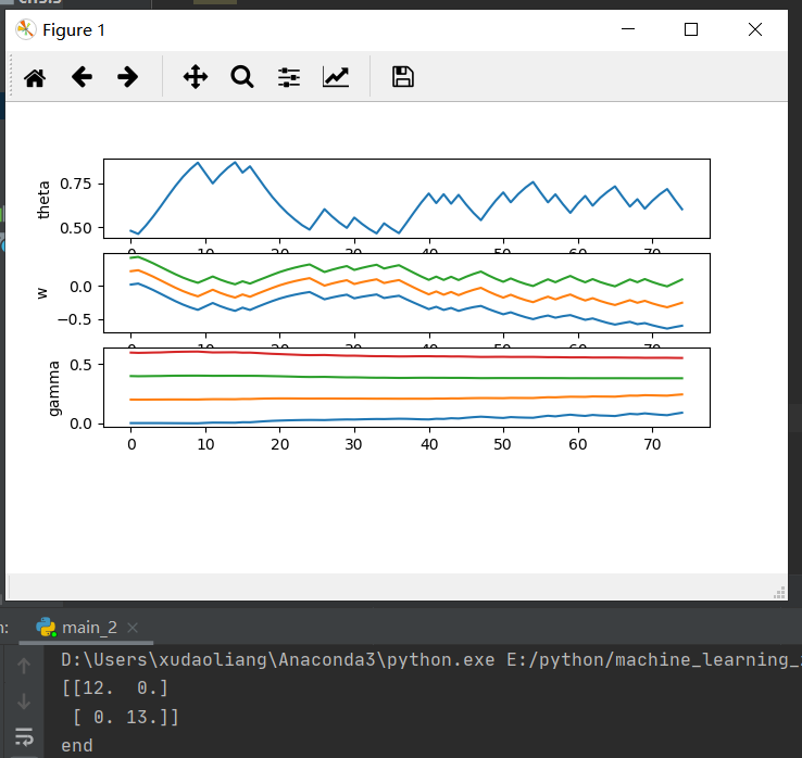
虽然准确率已经达到了100%,但是各个参数没有趋于稳定,这跟标准BP算法自身有很大的关系
心得
以下是自己改进程序的过程
#2、把三个神经元改为五个神经元
#3、调节eta2的值
#4、参数不再随机化赋值,改为赋指定值,每次都使用不同的初值,肯定不方便观察eta2对训练结果的影响
#5、初始参数赋指定值,调节eta2
#6、跟着程序一步一步的走,发现eta1的作用远比eta2大得多
进一步改进:简化函数主体的结构,并作出 precision = f(eta1,eta2)的图像,寻找合适的eta1和eta2