Clustering to Reduce Spatial Data Set Size

Read/cite the paper here.

In this tutorial, I demonstrate how to reduce the size of a spatial data set of GPS latitude-longitude coordinates using Python and its scikit-learn implementation of the DBSCAN clustering algorithm. All my code is in this IPython notebook in this GitHub repo, where you can also find the data.

Traditionally it’s been a problem that researchers did not have enough spatial data to answer useful questions or build compelling visualizations. Today, however, the problem is often that we have too much data. Too many scattered points on a map can overwhelm a viewer looking for a simple narrative. Furthermore, rendering a JavaScript web map (like Leaflet) with millions of data points on a mobile device can swamp the processor and be unresponsive.

 

The data set

How can we reduce the size of a data set down to a smaller set of spatially representative points? Consider a spatial data set with 1,759 latitude-longitude coordinates. This manageable data set is not too large to map, but it serves as a useful object for this tutorial (for a more complex example clustering 1.2 million GPS coordinates, see this project).

I have discussed this data set in a series of posts, and reverse-geocoded the coordinates to add city and country data. Here is a simple Python matplotlib scatter plot of all the coordinates in the full data set:

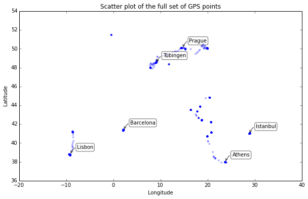
 At this scale, only a few dozen of the 1,759 data points are really visible. Even zoomed in very close, several locations have hundreds of data points stacked directly on top of each other due to the duration of time spent at one location. Unless we are interested in time dynamics, we simply do not need all of these spatially redundant points – they just bloat the data set’s size.

How much data do we need?

Look at the tight cluster of points representing Barcelona around the coordinate pair (2.15, 41.37). I stayed at the same place for a month and my GPS coordinates were recorded every 15 minutes, so I ended up with hundreds of rows in my data set corresponding to the coordinates of my apartment.

This high number of observations is useful for representing the duration of time spent at certain locations. However, it grows less useful if the objective is to represent merely where one has been. In that case only a single data point is needed for each geographical location to demonstrate that it has been visited. This reduced-size data set would be far easier to map with an on-the-fly rendering tool like JavaScript. It’s also far easier to reverse-geocode only the spatially representative points rather than the thousands or possibly millions of points in some full data set.

Clustering algorithms: k-means and DBSCAN

The k-means algorithm is likely the most common clustering algorithm. But for spatial data, the DBSCAN algorithm is far superior. Why?

The k-means algorithm groups N observations (i.e., rows in an array of coordinates) into k clusters. However, k-means is not an ideal algorithm for latitude-longitude spatial data because it minimizes variance, not geodetic distance. There is substantial distortion at latitudes far from the equator, like those of this data set. The algorithm would still “work” but its results are poor and there isn’t much that can be done to improve them.

With k-means, locations where I spent a lot of time – such as Barcelona – would still be over-represented because the initial random selection to seed the k-means algorithm would select them multiple times. Thus, more rows near a given location in the data set means a higher probability of having more rows selected randomly for that location. Even worse, due to the random seed, many locations would be missing from any clusters, and increasing the number of clusters would still leave patchy gaps throughout the reduced data set.

Instead, let’s use an algorithm that works better with arbitrary distances: scikit-learn’s implementation of the DBSCAN algorithm. DBSCAN clusters a spatial data set based on two parameters: a physical distance from each point, and a minimum cluster size. This method works much better for spatial latitude-longitude data.

Spatial data clustering with DBSCAN

Time to cluster. I begin by importing necessary Python modules and loading up the full data set. I convert the latitude and longitude coordinates’ columns into a two-dimensional numpy array, called coords:

import pandas as pd, numpy as np, matplotlib.pyplot as plt
from sklearn.cluster import DBSCAN
from geopy.distance import great_circle
from shapely.geometry import MultiPoint
df = pd.read_csv('summer-travel-gps-full.csv')
coords = df.as_matrix(columns=['lat', 'lon'])

Next I compute DBSCAN. The epsilon parameter is the max distance (1.5 km in this example) that points can be from each other to be considered a cluster. The min_samples parameter is the minimum cluster size (everything else gets classified as noise). I’ll set min_samples to 1 so that every data point gets assigned to either a cluster or forms its own cluster of 1. Nothing will be classified as noise.

I use the haversine metric and ball tree algorithm to calculate great circle distances between points. Notice my epsilon and coordinates get converted to radians, because scikit-learn’s haversine metric needs radian units:

kms_per_radian = 6371.0088
epsilon = 1.5 / kms_per_radian
db = DBSCAN(eps=epsilon, min_samples=1, algorithm='ball_tree', metric='haversine').fit(np.radians(coords))
cluster_labels = db.labels_
num_clusters = len(set(cluster_labels))
clusters = pd.Series([coords[cluster_labels == n] for n in range(num_clusters)])
print('Number of clusters: {}'.format(num_clusters))

Ok, now I’ve got 138 clusters. Unlike k-means, DBSCAN doesn’t require you to specify the number of clusters in advance – it determines them automatically based on the epsilon and min_samples parameters.

Finding a cluster’s center-most point

To reduce my data set size, I want to grab the coordinates of one point from each cluster that was formed. I could just take the first point in each cluster, but it would be more spatially-representative if I take the point nearest the cluster’s centroid. Note that with DBSCAN, clusters may be non-convex and centers may fall outside the cluster – however, we just want to reduce the cluster down to a single point. The point nearest its center is perfectly suitable for this.

This function returns the center-most point from a cluster by taking a set of points (i.e., a cluster) and returning the point within it that is nearest to some reference point (in this case, the cluster’s centroid):

def get_centermost_point(cluster):
    centroid = (MultiPoint(cluster).centroid.x, MultiPoint(cluster).centroid.y)
    centermost_point = min(cluster, key=lambda point: great_circle(point, centroid).m)
    return tuple(centermost_point)
centermost_points = clusters.map(get_centermost_point)

The function above first calculates the centroid’s coordinates. Then I use Python’s built-in min function to find the smallest member of the cluster in terms of distance to that centroid. The key argument does this with a lambda function that calculates each point’s distance to the centroid in meters, via geopy’s great circle function. Finally, I return the coordinates of the point that was the least distance from the centroid.

To use this function, I map it to my pandas series of clusters. In other words, for each element (i.e., cluster) in the series, it gets the center-most point and then assembles all these center-most points into a new series called centermost_points. Then I turn these center-most points into a pandas dataframe of points which are spatially representative of my clusters (and in turn, my original full data set):

lats, lons = zip(*centermost_points)
rep_points = pd.DataFrame({'lon':lons, 'lat':lats})

Great! Now I’ve got my set of 138 spatially representative points. But, I also want the city, country, and date information that was contained in the original full data set. So, for each row of representative points, I pull the full row from the original data set where the latitude and longitude columns match the representative point’s latitude and longitude:

rs = rep_points.apply(lambda row: df[(df['lat']==row['lat']) && (df['lon']==row['lon'])].iloc[0], axis=1)

All done. I’ve reduced my original data set down to a spatially representative set of points with full details.

Final result from DBSCAN

I’ll plot the final reduced set of data points versus the original full set to see how they compare:

fig, ax = plt.subplots(figsize=[10, 6])
rs_scatter = ax.scatter(rs['lon'], rs['lat'], c='#99cc99', edgecolor='None', alpha=0.7, s=120)
df_scatter = ax.scatter(df['lon'], df['lat'], c='k', alpha=0.9, s=3)
ax.set_title('Full data set vs DBSCAN reduced set')
ax.set_xlabel('Longitude')
ax.set_ylabel('Latitude')
ax.legend([df_scatter, rs_scatter], ['Full set', 'Reduced set'], loc='upper right')
plt.show()

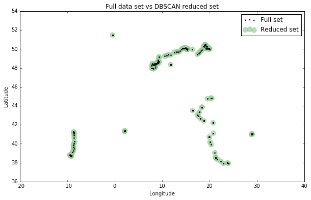
 Looks good! You can see the 138 representative points, in green, approximating the spatial distribution of the 1,759 points of the full data set, in black. DBSCAN reduced the data by 92.2%, from 1,759 points to 138 points. There are no gaps in the reduced data set and heavily-trafficked spots (like Barcelona) are no longer drastically over-represented.

出处：Clustering to Reduce Spatial Data Set Size – Geoff Boeing