【转载】用OCTAVE实现一元线性回归的梯度下降算法

Posted on 2018-01-14 22:57 西瓜K菠萝阅读(365) 评论(0) 编辑收藏举报

原文地址：http://www.cnblogs.com/KID-XiaoYuan/p/7247481.html

STEP1 PLOTTING THE DATA

在处理数据之前，我们通常要了解数据，对于这次的数据集合，我们可以通过离散的点来描绘它，在一个2D的平面里把它画出来。

ex1data1.txt

我们把ex1data1中的内容读取到X变量和y变量中，用m表示数据长度。

data = load('ex1data1.txt');
X = data(:,1);
y = data(:,2);
m = length(y);

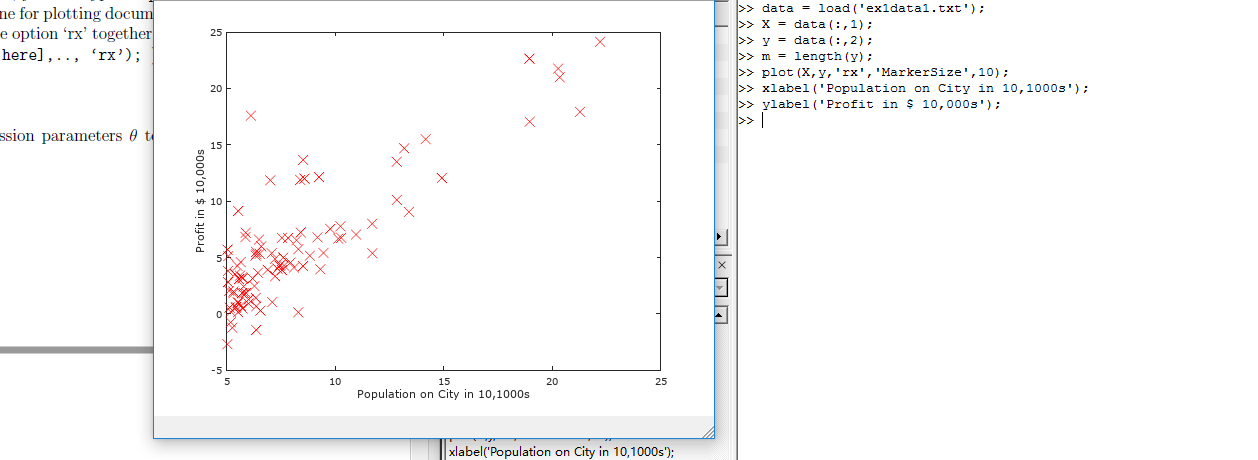
接下来通过图像描绘出来。

plot(x,y,'rx','MakerSize',10);
ylabel('Profit in $10,000s');
xlabel('Population of City in 10,000s');

　　现在我们得到图像如图所示，就是原始的数据的直观表示。

STEP2 GRADIENT DESCENT

现在，我们通过梯度下降法对参数θ进行线性回归。

依照我们之前所得出步骤方法

迭代更新

计算θ值函数：

function J = computeCost(X, y, theta)
%COMPUTECOST Compute cost for linear regression
%   J = COMPUTECOST(X, y, theta) computes the cost of using theta as the
%   parameter for linear regression to fit the data points in X and y
 
% Initialize some useful values
m = length(y); % number of training examples
 
% You need to return the following variables correctly
J = 0;
 
% ====================== YOUR CODE HERE ======================
% Instructions: Compute the cost of a particular choice of theta
%               You should set J to the cost.
J = sum((X * theta - y).^2) / (2*m);     % X(79,2)  theta(2,1)
 
 
 
 
 
% =========================================================================
 
end

　　接下来是梯度下降函数

function [theta, J_history] = gradientDescent(X, y, theta, alpha, num_iters)
%GRADIENTDESCENT Performs gradient descent to learn theta
%   theta = GRADIENTDESENT(X, y, theta, alpha, num_iters) updates theta by
%   taking num_iters gradient steps with learning rate alpha
 
% Initialize some useful values
m = length(y); % number of training examples
J_history = zeros(num_iters, 1);
theta_s=theta;
 
for iter = 1:num_iters
 
    % ====================== YOUR CODE HERE ======================
    % Instructions: Perform a single gradient step on the parameter vector
    %               theta.
    %
    % Hint: While debugging, it can be useful to print out the values
    %       of the cost function (computeCost) and gradient here.
    %
    theta(1) = theta(1) - alpha / m * sum(X * theta_s - y);      
    theta(2) = theta(2) - alpha / m * sum((X * theta_s - y) .* X(:,2));    
% 必须同时更新theta(1)和theta(2)，所以不能用X * theta,而要用theta_s存储上次结果。
    theta_s=theta;
     
 
    % ============================================================
 
    % Save the cost J in every iteration   
    J_history(iter) = computeCost(X, y, theta);
 
end
J_history
end

绘图函数：

function plotData(x, y)
%PLOTDATA Plots the data points x and y into a new figure
% PLOTDATA(x,y) plots the data points and gives the figure axes labels of
% population and profit.
 
% ====================== YOUR CODE HERE ======================
% Instructions: Plot the training data into a figure using the
% "figure" and "plot" commands. Set the axes labels using
% the "xlabel" and "ylabel" commands. Assume the
% population and revenue data have been passed in
% as the x and y arguments of this function.
%
% Hint: You can use the 'rx' option with plot to have the markers
% appear as red crosses. Furthermore, you can make the
% markers larger by using plot(..., 'rx', 'MarkerSize', 10);
 
figure; % open a new figure window
plot(x, y, 'rx', 'MarkerSize', 10); % Plot the data
ylabel('Profit in $10,000s'); % Set the y axis label
xlabel('Population of City in 10,000s'); % Set the x axis label
 
  
 
  
 
% ============================================================
 
end

　　　　根据以上函数，我们进行线性回归：

<br>%% Machine Learning Online Class - Exercise 1: Linear Regression
 
%  Instructions
%  ------------
%
%  This file contains code that helps you get started on the
%  linear exercise. You will need to complete the following functions
%  in this exericse:
%
%     warmUpExercise.m
%     plotData.m
%     gradientDescent.m
%     computeCost.m
%     gradientDescentMulti.m
%     computeCostMulti.m
%     featureNormalize.m
%     normalEqn.m
%
%  For this exercise, you will not need to change any code in this file,
%  or any other files other than those mentioned above.
%
% x refers to the population size in 10,000s
% y refers to the profit in $10,000s
%
 
 
%% ==================== Part 1: Basic Function ====================
% Complete warmUpExercise.m
fprintf('Running warmUpExercise ... \n');
fprintf('5x5 Identity Matrix: \n');
warmUpExercise()
 
fprintf('Program paused. Press enter to continue.\n');
pause;
 
 
%% ======================= Part 2: Plotting =======================
fprintf('Plotting Data ...\n')
data = load('ex1data1.txt');
X = data(:, 1); y = data(:, 2);
m = length(y); % number of training examples
 
% Plot Data
% Note: You have to complete the code in plotData.m
plotData(X, y);
 
fprintf('Program paused. Press enter to continue.\n');
pause;
 
%% =================== Part 3: Gradient descent ===================
fprintf('Running Gradient Descent ...\n')
 
X = [ones(m, 1), data(:,1)]; % Add a column of ones to x
theta = zeros(2, 1); % initialize fitting parameters
 
% Some gradient descent settings
iterations = 1500;
alpha = 0.01;
 
% compute and display initial cost
computeCost(X, y, theta)
 
% run gradient descent
theta = gradientDescent(X, y, theta, alpha, iterations);
 
% print theta to screen
fprintf('Theta found by gradient descent: ');
fprintf('%f %f \n', theta(1), theta(2));
 
% Plot the linear fit
hold on; % keep previous plot visible
plot(X(:,2), X*theta, '-')
legend('Training data', 'Linear regression')
hold off % don't overlay any more plots on this figure
 
% Predict values for population sizes of 35,000 and 70,000
predict1 = [1, 3.5] *theta;
fprintf('For population = 35,000, we predict a profit of %f\n',...
    predict1*10000);
predict2 = [1, 7] * theta;
fprintf('For population = 70,000, we predict a profit of %f\n',...
    predict2*10000);
 
fprintf('Program paused. Press enter to continue.\n');
pause;
 
%% ============= Part 4: Visualizing J(theta_0, theta_1) =============
fprintf('Visualizing J(theta_0, theta_1) ...\n')
 
% Grid over which we will calculate J
theta0_vals = linspace(-10, 10, 100);
theta1_vals = linspace(-1, 4, 100);
 
% initialize J_vals to a matrix of 0's
J_vals = zeros(length(theta0_vals), length(theta1_vals));
 
% Fill out J_vals
for i = 1:length(theta0_vals)
    for j = 1:length(theta1_vals)
      t = [theta0_vals(i); theta1_vals(j)];   
      J_vals(i,j) = computeCost(X, y, t);
    end
end
 
 
% Because of the way meshgrids work in the surf command, we need to
% transpose J_vals before calling surf, or else the axes will be flipped
J_vals = J_vals';
% Surface plot
figure;
surf(theta0_vals, theta1_vals, J_vals)
xlabel('\theta_0'); ylabel('\theta_1');
 
% Contour plot
figure;
% Plot J_vals as 15 contours spaced logarithmically between 0.01 and 100
contour(theta0_vals, theta1_vals, J_vals, logspace(-2, 3, 20))
xlabel('\theta_0'); ylabel('\theta_1');
hold on;
plot(theta(1), theta(2), 'rx', 'MarkerSize', 10, 'LineWidth', 2);

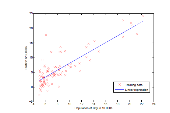
如图所示，绘制出线性回归函数。

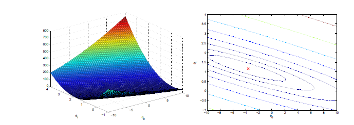
这时所绘制2D等高线图梯度下降表面图：

function [X_norm, mu, sigma] = featureNormalize(X)
%FEATURENORMALIZE Normalizes the features in X
%   FEATURENORMALIZE(X) returns a normalized version of X where
%   the mean value of each feature is 0 and the standard deviation
%   is 1. This is often a good preprocessing step to do when
%   working with learning algorithms.
 
% You need to set these values correctly
X_norm = X;
mu = zeros(1, size(X, 2));      % mean value 均值   size(X,2)  列数
sigma = zeros(1, size(X, 2));   % standard deviation  标准差
 
% ====================== YOUR CODE HERE ======================
% Instructions: First, for each feature dimension, compute the mean
%               of the feature and subtract it from the dataset,
%               storing the mean value in mu. Next, compute the
%               standard deviation of each feature and divide
%               each feature by it's standard deviation, storing
%               the standard deviation in sigma.
%
%               Note that X is a matrix where each column is a
%               feature and each row is an example. You need
%               to perform the normalization separately for
%               each feature.
%
% Hint: You might find the 'mean' and 'std' functions useful.
%      
  mu = mean(X);       %  mean value
  sigma = std(X);     %  standard deviation
  X_norm  = (X - repmat(mu,size(X,1),1)) ./  repmat(sigma,size(X,1),1);
  
 
 
 
 
 
 
 
% ============================================================
 
end
function [theta, J_history] = gradientDescentMulti(X, y, theta, alpha, num_iters)
%GRADIENTDESCENTMULTI Performs gradient descent to learn theta
%   theta = GRADIENTDESCENTMULTI(x, y, theta, alpha, num_iters) updates theta by
%   taking num_iters gradient steps with learning rate alpha
 
% Initialize some useful values
m = length(y); % number of training examples
J_history = zeros(num_iters, 1);
 
for iter = 1:num_iters
 
    % ====================== YOUR CODE HERE ======================
    % Instructions: Perform a single gradient step on the parameter vector
    %               theta.
    %
    % Hint: While debugging, it can be useful to print out the values
    %       of the cost function (computeCostMulti) and gradient here.
    %
    theta = theta - alpha / m * X' * (X * theta - y);
 
 
    % ============================================================
 
    % Save the cost J in every iteration   
    J_history(iter) = computeCostMulti(X, y, theta);
 
end
 
end
function J = computeCostMulti(X, y, theta)
%COMPUTECOSTMULTI Compute cost for linear regression with multiple variables
%   J = COMPUTECOSTMULTI(X, y, theta) computes the cost of using theta as the
%   parameter for linear regression to fit the data points in X and y
 
% Initialize some useful values
m = length(y); % number of training examples
 
% You need to return the following variables correctly
J = 0;
 
% ====================== YOUR CODE HERE ======================
% Instructions: Compute the cost of a particular choice of theta
%               You should set J to the cost.
J = sum((X * theta - y).^2) / (2*m);   
 
 
 
 
% =========================================================================
 
end
function [theta] = normalEqn(X, y)
%NORMALEQN Computes the closed-form solution to linear regression
%   NORMALEQN(X,y) computes the closed-form solution to linear
%   regression using the normal equations.
 
theta = zeros(size(X, 2), 1);
 
% ====================== YOUR CODE HERE ======================
% Instructions: Complete the code to compute the closed form solution
%               to linear regression and put the result in theta.
%
 
% ---------------------- Sample Solution ----------------------
 
theta = pinv( X' * X ) * X' * y;
 
 
% -------------------------------------------------------------
 
 
% ============================================================
 
end
%% Machine Learning Online Class
%  Exercise 1: Linear regression with multiple variables
%
%  Instructions
%  ------------
%
%  This file contains code that helps you get started on the
%  linear regression exercise.
%
%  You will need to complete the following functions in this
%  exericse:
%
%     warmUpExercise.m
%     plotData.m
%     gradientDescent.m
%     computeCost.m
%     gradientDescentMulti.m
%     computeCostMulti.m
%     featureNormalize.m
%     normalEqn.m
%
%  For this part of the exercise, you will need to change some
%  parts of the code below for various experiments (e.g., changing
%  learning rates).
%
 
%% Initialization
 
%% ================ Part 1: Feature Normalization ================
 
%% Clear and Close Figures
clear ; close all; clc
 
fprintf('Loading data ...\n');
 
%% Load Data
data = load('ex1data2.txt');
X = data(:, 1:2);
y = data(:, 3);
m = length(y);
 
% Print out some data points
fprintf('First 10 examples from the dataset: \n');
fprintf(' x = [%.0f %.0f], y = %.0f \n', [X(1:10,:) y(1:10,:)]');
 
fprintf('Program paused. Press enter to continue.\n');
pause;
 
% Scale features and set them to zero mean
fprintf('Normalizing Features ...\n');
 
[X mu sigma] = featureNormalize(X);      % 均值0，标准差1
 
% Add intercept term to X
X = [ones(m, 1) X];
 
 
%% ================ Part 2: Gradient Descent ================
 
% ====================== YOUR CODE HERE ======================
% Instructions: We have provided you with the following starter
%               code that runs gradient descent with a particular
%               learning rate (alpha).
%
%               Your task is to first make sure that your functions -
%               computeCost and gradientDescent already work with
%               this starter code and support multiple variables.
%
%               After that, try running gradient descent with
%               different values of alpha and see which one gives
%               you the best result.
%
%               Finally, you should complete the code at the end
%               to predict the price of a 1650 sq-ft, 3 br house.
%
% Hint: By using the 'hold on' command, you can plot multiple
%       graphs on the same figure.
%
% Hint: At prediction, make sure you do the same feature normalization.
%
 
fprintf('Running gradient descent ...\n');
 
% Choose some alpha value
alpha = 0.01;
num_iters = 8500;
 
% Init Theta and Run Gradient Descent
theta = zeros(3, 1);
[theta, J_history] = gradientDescentMulti(X, y, theta, alpha, num_iters);
 
% Plot the convergence graph
figure;
plot(1:numel(J_history), J_history, '-b', 'LineWidth', 2);
xlabel('Number of iterations');
ylabel('Cost J');
 
% Display gradient descent's result
fprintf('Theta computed from gradient descent: \n');
fprintf(' %f \n', theta);
fprintf('\n');
 
% Estimate the price of a 1650 sq-ft, 3 br house
% ====================== YOUR CODE HERE ======================
% Recall that the first column of X is all-ones. Thus, it does
% not need to be normalized.
price = [1 (([1650 3]-mu) ./ sigma)] * theta ;
% ============================================================
 
fprintf(['Predicted price of a 1650 sq-ft, 3 br house ' ...
         '(using gradient descent):\n $%f\n'], price);
 
fprintf('Program paused. Press enter to continue.\n');
pause;
 
%% ================ Part 3: Normal Equations ================
 
fprintf('Solving with normal equations...\n');
 
% ====================== YOUR CODE HERE ======================
% Instructions: The following code computes the closed form
%               solution for linear regression using the normal
%               equations. You should complete the code in
%               normalEqn.m
%
%               After doing so, you should complete this code
%               to predict the price of a 1650 sq-ft, 3 br house.
%
 
%% Load Data
data = csvread('ex1data2.txt');
X = data(:, 1:2);
y = data(:, 3);
m = length(y);
 
% Add intercept term to X
X = [ones(m, 1) X];
 
% Calculate the parameters from the normal equation
theta = normalEqn(X, y);
 
% Display normal equation's result
fprintf('Theta computed from the normal equations: \n');
fprintf(' %f \n', theta);
fprintf('\n');
 
 
% Estimate the price of a 1650 sq-ft, 3 br house
% ====================== YOUR CODE HERE ======================
price = [1 1650 3] * theta ;
 
 
% ============================================================
 
fprintf(['Predicted price of a 1650 sq-ft, 3 br house ' ...
         '(using normal equations):\n $%f\n'], price);

　　处理前：

处理后：

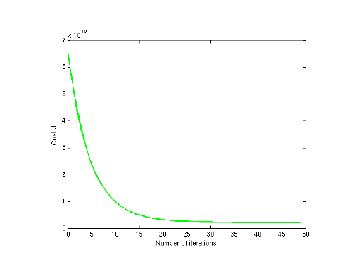
回归过程如图所示：

至此，我们通过梯度下降法解决了此问题，我们还可以通过之前所说的数学方法来解决，但是对于数据太大的情况（通常大于10000），我们就会通过梯度下降法来解决了

　　根据以上函数，我们进行线性回归：

刷新页面返回顶部

Jincw! A za A za Fighting!

公告

【转载】用OCTAVE实现一元线性回归的梯度下降算法

STEP1 PLOTTING THE DATA

STEP2 GRADIENT DESCENT