如何判别模型的优劣？

引言

　　选择用于评估机器学习算法的指标非常重要。度量的选择会影响如何测量和比较机器学习算法的性能。它们会影响您如何权衡结果中不同特征的重要性以及您选择哪种算法的最终选择。在这篇文章中，您将了解如何使用scikit-learn在Python中选择和使用不同的机器学习性能指标。

回归问题：

平均绝对误差
均方误差
均方根误差
R²

分类问题：

Classification Accuracy 分类问题准确率
Logarithmic Loss 对数损失函数
Confusion Matrix 混淆矩阵
Area Under ROC Curve ROC曲线下的面积
Classification Report 分类报告

更多参考：here

回归问题

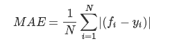
平均绝对误差（Mean Absolute Error）

　　平均绝对误差（MAE）是预测值与实际值之间的绝对差值之和。该度量给出了误差幅度的概念，但不知道方向（例如，过度或低于预测），MSE可以评价数据的变化程度，MSE的值越小，说明预测模型描述实验数据具有更好的精确度。

以下示例演示了计算波士顿房价数据集的平均绝对误差。

# Cross Validation Regression MAE
import pandas
from sklearn import model_selection
from sklearn.linear_model import LinearRegression

url = "https://raw.githubusercontent.com/jbrownlee/Datasets/master/housing.data"
names = ['CRIM', 'ZN', 'INDUS', 'CHAS', 'NOX', 'RM', 'AGE', 'DIS', 'RAD', 'TAX', 'PTRATIO', 'B', 'LSTAT', 'MEDV']

dataframe = pandas.read_csv(url, delim_whitespace=True, names=names)
array = dataframe.values
X = array[:,0:13]
Y = array[:,13]
seed = 7
kfold = model_selection.KFold(n_splits=10, random_state=seed)
model = LinearRegression()
scoring = 'neg_mean_absolute_error'
results = model_selection.cross_val_score(model, X, Y, cv=kfold, scoring=scoring)
print(("MAE: (%.3f.) (%.3f.)") % (results.mean(), results.std()))

MAE: (-4.005.) (2.084.

均方误差(Mean Squared Error)

　　MSE是参数估计值与参数真值之差的平方的期望值

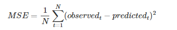
这个应用应该是最广的，因为他能够求导，所以经常作为loss function。计算的结果就是你的预测值和真实值的差距的平方和。

# Cross Validation Regression MSE
import pandas
from sklearn import model_selection
from sklearn.linear_model import LinearRegression
url = "https://raw.githubusercontent.com/jbrownlee/Datasets/master/housing.data"
names = ['CRIM', 'ZN', 'INDUS', 'CHAS', 'NOX', 'RM', 'AGE', 'DIS', 'RAD', 'TAX', 'PTRATIO', 'B', 'LSTAT', 'MEDV']
dataframe = pandas.read_csv(url, delim_whitespace=True, names=names)
array = dataframe.values
X = array[:,0:13]
Y = array[:,13]
seed = 7
kfold = model_selection.KFold(n_splits=10, random_state=seed)
model = LinearRegression()
scoring = 'neg_mean_squared_error'
results = model_selection.cross_val_score(model, X, Y, cv=kfold, scoring=scoring)
print(("MSE: (%.3f.) (%.3f.)") % (results.mean(), results.std()))

MSE: (-34.705.) (45.574.)

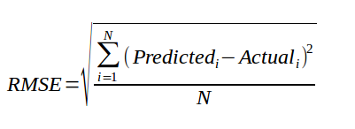
均方根误差(Root Mean Square Error)

均方根值（RMSE）：也称方均根值或有效值，它的计算方法是先平方、再平均、然后开方。

是观测值与真值偏差的平方和与观测次数m比值的平方根。
是用来衡量观测值同真值之间的偏差

R²

R ^ 2（或R Squared）度量提供了一组预测与实际值的拟合优度的指示。在统计文献中，该度量被称为可决系数。对于不适合和完美贴合，这是介于0和1之间的值。

表达式：R2=SSR/SST=1-SSE/SST

其中：SST=SSR+SSE，SST(total sum of squares)为总平方和，SSR(regression sum of squares)为回归平方和，SSE(error sum of squares) 为残差平方和。

以下示例提供了计算一组预测的平均R ^ 2的演示.

import pandas
from sklearn import model_selection
from sklearn.linear_model import LinearRegression
url = "https://raw.githubusercontent.com/jbrownlee/Datasets/master/housing.data"
names = ['CRIM', 'ZN', 'INDUS', 'CHAS', 'NOX', 'RM', 'AGE', 'DIS', 'RAD', 'TAX', 'PTRATIO', 'B', 'LSTAT', 'MEDV']
dataframe = pandas.read_csv(url, delim_whitespace=True, names=names)
array = dataframe.values
X = array[:,0:13]
Y = array[:,13]
seed = 7
kfold = model_selection.KFold(n_splits=10, random_state=seed)
model = LinearRegression()
scoring = 'r2'
results = model_selection.cross_val_score(model, X, Y, cv=kfold, scoring=scoring)
print(("R^2: (%.3f.） (%.3f.)") % (results.mean(), results.std()))

R^2: (0.203.） (0.595.)

note:scoring可选

['accuracy', 'adjusted_mutual_info_score', 'adjusted_rand_score', 'average_precision', 
'completeness_score', 'explained_variance', 'f1', 'f1_macro', 'f1_micro', 'f1_samples', 'f1_weighted', 'fowlkes_mallows_score', 'homogeneity_score', 'mutual_info_score', 
'neg_log_loss', 'neg_mean_absolute_error', 'neg_mean_squared_error', 'neg_mean_squared_log_error', 'neg_median_absolute_error', 'normalized_mutual_info_score', 'precision', 
'precision_macro', 'precision_micro', 'precision_samples', 'precision_weighted', 'r2', 'recall', 'recall_macro', 'recall_micro', 'recall_samples', 'recall_weighted', 'roc_auc',
 'v_measure_score']

分类问题

分类的准确率（Classification Accuracy ）

确定准确度是作为所有预测的比率而作出的正确预测的数量。

这是分类问题最常见的评估指标，也是最常用的评估指标。它实际上只适用于每个类别中观察数量相同的情况（很少这种情况），并且所有预测和预测误差都同样重要。

以下是计算分类准确度的示例。

# Cross Validation Classification Accuracy
import pandas
from sklearn import model_selection
from sklearn.linear_model import LogisticRegression
url = "https://raw.githubusercontent.com/jbrownlee/Datasets/master/pima-indians-diabetes.data.csv"
names = ['preg', 'plas', 'pres', 'skin', 'test', 'mass', 'pedi', 'age', 'class']
dataframe = pandas.read_csv(url, names=names)
array = dataframe.values
X = array[:,0:8]
Y = array[:,8]
seed = 7
kfold = model_selection.KFold(n_splits=10, random_state=seed)
model = LogisticRegression()
scoring = 'accuracy'
results = model_selection.cross_val_score(model, X, Y, cv=kfold, scoring=scoring)
print(("Accuracy: (%.3f.) (%.3f.)") % (results.mean(), results.std()))

Accuracy: (0.770.) (0.048.)

对数损失函数（Logarithmic Loss）

对数损失（或logloss）是用于评估给定类的成员概率的预测的性能度量。可以将0和1之间的标量概率视为对算法预测的置信度的度量。正确或不正确的预测会与预测的置信度成比例地得到奖励或惩罚。

以下是计算Pima Indians糖尿病数据集开始时Logistic回归预测的logloss的示例。

# Cross Validation Classification LogLoss
import pandas
from sklearn import model_selection
from sklearn.linear_model import LogisticRegression
url = "https://raw.githubusercontent.com/jbrownlee/Datasets/master/pima-indians-diabetes.data.csv"
names = ['preg', 'plas', 'pres', 'skin', 'test', 'mass', 'pedi', 'age', 'class']
dataframe = pandas.read_csv(url, names=names)
array = dataframe.values
X = array[:,0:8]
Y = array[:,8]
seed = 7
kfold = model_selection.KFold(n_splits=10, random_state=seed)
model = LogisticRegression()
scoring = 'neg_log_loss'
results = model_selection.cross_val_score(model, X, Y, cv=kfold, scoring=scoring)
print(("Logloss:( %.3f.) (%.3f.)") % (results.mean(), results.std()))

Logloss:( -0.492.) (0.047.)

混淆矩阵（Confusion Matrix）

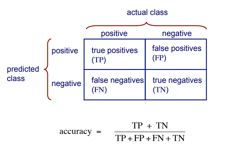
　　混淆矩阵是具有两个或更多类的模型的准确性的便利表示。该表提供了关于x轴的预测和y轴上的准确度结果。表格的单元格是机器学习算法所做的预测次数。

例如，机器学习算法可以预测0或1，并且每个预测实际上可以是0或1.对于0的实际为0的预测出现在用于预测的单元格中= 0并且实际= 0，而对于0的预测是0 实际上1出现在单元格中，用于预测= 0和实际= 1。

其中，精准率（accracy），召回率（recall）和F1得分将在分类报告中给出。

# Cross Validation Classification Confusion Matrix
import pandas
from sklearn import model_selection
from sklearn.linear_model import LogisticRegression
from sklearn.metrics import confusion_matrix

url = "https://raw.githubusercontent.com/jbrownlee/Datasets/master/pima-indians-diabetes.data.csv"
names = ['preg', 'plas', 'pres', 'skin', 'test', 'mass', 'pedi', 'age', 'class']
dataframe = pandas.read_csv(url, names=names)
array = dataframe.values

X = array[:,0:8]
Y = array[:,8]

test_size = 0.33
seed = 7
X_train, X_test, Y_train, Y_test = model_selection.train_test_split(X, Y, test_size=test_size, random_state=seed)
logreg = LogisticRegression()
logreg.fit(X_train, Y_train)

LogisticRegression(C=1.0, class_weight=None, dual=False, fit_intercept=True,

          intercept_scaling=1, max_iter=100, multi_class='ovr', n_jobs=1,
          penalty='l2', random_state=None, solver='liblinear', tol=0.0001,
          verbose=0, warm_start=False)

# make class predictions for the testing set
y_pred_class = logreg.predict(X_test)

分类准确度（Classification accuracy）：正确预测的百分比

# calculate accuracy
from sklearn import metrics
print(metrics.accuracy_score(Y_test, y_pred_class))

0.7559055118110236

分类准确率为69％。

混淆矩阵（Confusion Matrix）

matrix = confusion_matrix(Y_test, y_pred_class)
print(matrix)

[[141  21]
 [ 41  51]]

n =

Predicted:

Actual:

141

Actual:

测试集中的每个观察都只用一个框表示,它是一个2x2矩阵，因为有2个响应类.

注意：此处的矩阵与图的格式并不一致。

基本术语

真阳性（True Positive,,TP）：我们正确地预测他们确实患有糖尿病
51
真阴性（Ture Negatives,TN）：我们正确地预测他们没有糖尿病
141
误报（False Positives，FP）：我们错误地预测他们确实患有糖尿病（“I型错误”）
21
虚假地预测积极的
输入I错误
假阴性（False Negatives,FN）：我们错误地预测他们没有糖尿病（“II型错误”）
41
虚假地预测消极
II型错误

0: negative class
1: positive class

# save confusion matrix and slice into four pieces
confusion = metrics.confusion_matrix(Y_test, y_pred_class)
print(confusion)
#[row, column]
TP = confusion[1, 1]
TN = confusion[0, 0]
FP = confusion[0, 1]
FN = confusion[1, 0]


[[141  21]
 [ 41  51]]

根据混淆矩阵计算度量

分类准确度

# use float to perform true division, not integer division
print((TP + TN) / float(TP + TN + FP + FN))
#用于对比
print(metrics.accuracy_score(Y_test, y_pred_class))

0.7559055118110236
0.7559055118110236

结果一致 .

分类错误（Classification Error）

也被称为误分类率（Misclassification Rate）

classification_error = (FP + FN) / float(TP + TN + FP + FN)

print(classification_error)
print(1 - metrics.accuracy_score(Y_test, y_pred_class))

0.2440944881889764
0.2440944881889764

灵敏度（Sensitivity）

灵敏度（Sensitivity）：当实际值为正时，预测的正确频率是多少？即分类正确的正样本个数占正样本个数的比例。我们想要最大化的东西，检测正面实例的分类器有多“敏感”。

也被称为“真正的正面率（True Positive Rate）”或“召回率（Recall）”

TP /全部为阳性
- - Rcall= TP / TP + FN

sensitivity = TP / float(FN + TP)

print(sensitivity)
print(metrics.recall_score(Y_test, y_pred_class))


0.5543478260869565
0.5543478260869565

特异性（Specificity）

特异性：当实际值为负时，预测正确的频率是多少？即分类正确的负样本个数占负样本个数的比例我们想要最大化的东西，在预测正面实例时，“特定”（或“选择性”）是如何分类的？

TN /全部为负数

TN= TN + FP

specificity = TN / (TN + FP)

print(specificity)

0.8703703703703703

可以看出，我们的分类器：高特异性，不灵敏。

误报率（False Positive Rate）

误报率：当实际值为负时，预测错误的频率是多少？即分类错误的正样本个数占总分类错误样本个数的比例。

false_positive_rate = FP / float(TN + FP)

print(false_positive_rate)
print(1 - specificity)

0.12962962962962962
0.12962962962962965

精度(Precision)

精度：预测正值时，预测的正确频率是多少？

在预测正面实例时，分类器的“精确”程度如何？

precision = TP / float(TP + FP)

print(precision)
print(metrics.precision_score(Y_test, y_pred_class))

0.7083333333333334
0.7083333333333334

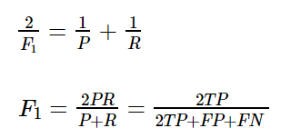
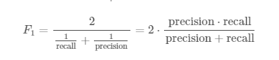
F1得分

以上讨论了precise（精确率）recall（召回率），接下来将使用一个新的机器学习指标F1分数，F1分数会同时考虑精确率和回召率，以便重新计算新的分数。

F1分数可以理解为：精确率和召回率的加权平均值。其中F1分数的最佳为1，最差为0；

F1 = 2 * (precise * recall) / (precise + recall)

f1_score = 2*( precision*sensitivity)/(precision+sensitivity)

print(f1_score)
print(metrics.f1_score(Y_test, y_pred_class))

0.6219512195121951
0.6219512195121951

宏F1得分（Macro F1）

我们已经知道，标准F1分数，即精度和召回的调和平均值：

对于多类问题，我们必须平均每个类的F1分数。宏观F1分数平均每个级别的F1分数，而不考虑标签不平衡。

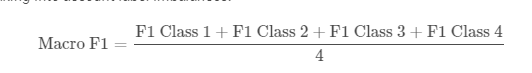
换句话说，当使用宏时，每个标签的出现次数不计入计算中.

有关差异的更多信息，请查看针对F1分数的Scikit-Learn文档 (Scikit-Learn Documention for F1 Score ) 或Stack Exchange问题和答案Stack Exchange question and answers.

from sklearn.metrics import f1_score
f1_score(y_true, y_predicted, average = 'macro`)

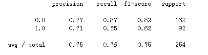
分类报告

分类报告可以方便简洁的帮助我们得到各项指标

report=metrics.classification_report(Y_test, y_pred_class)
print(report)

更进一步

据混淆矩阵计算度量，调整分类阈值（threshold）。

# print the first 10 predicted responses
# 1D array (vector) of binary values (0, 1)
logreg.predict(X_test)[0:10]

array([0., 1., 1., 0., 0., 0., 0., 0., 1., 0.])

# print the first 10 predicted probabilities of class membership
logreg.predict_proba(X_test)[0:10]

从直接的结果到概率的输出，可以更直观看到概率情况。

预测概率的重要性

我们可以根据糖尿病的概率对观察结果进排序，优先选择那些概率更高的人。

分类阈值为0.5

如果概率> 0.5，则预测1级
如果概率<0.5，则预测0级

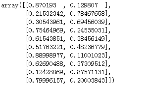
# print the first 10 predicted probabilities for class 1
logreg.predict_proba(X_test)[0:10, 1]

array([0.129807  , 0.78467658, 0.69456039, 0.24535031, 0.38456149,
       0.48236779, 0.11001023, 0.37309512, 0.87571131, 0.20003843])

# store the predicted probabilities for class 1
y_pred_prob = logreg.predict_proba(X_test)[:, 1]

# allow plots to appear in the notebook

import matplotlib.pyplot as plt

# adjust the font size 
plt.rcParams['font.size'] = 12

# histogram of predicted probabilities

# 10 bins
plt.hist(y_pred_prob,bins=10)

# x-axis limit from 0 to 1
plt.xlim(0,1)
plt.title('Histogram of predicted probabilities')
plt.xlabel('Predicted probability of diabetes')
plt.ylabel('Frequency')

我们可以从第三个栏看到：

大约45％的观测值的概率从0.2到0.3
少量观察概率> 0.5
这低于0.5的阈值
在这种情况下，大多数人会被预测为“无糖尿病”

解决办法

降低预测糖尿病的阈值（threshold）
增加分类器的灵敏度(sensitivity)

这会增加TP的数量
对积极情况更敏感

# sensitivity has increased (used to be 0.87)
print (81 / float(81 + 11))

# specificity has decreased (used to be 0.55)
print(101 / float(101 + 61))

# predict diabetes if the predicted probability is greater than 0.3
from sklearn.preprocessing import binarize
# it will return 1 for all values above 0.3 and 0 otherwise
# results are 2D so we slice out the first column
y_pred_class = binarize(y_pred_prob.reshape(1,-1), 0.3)[0]


# print the first 10 predicted probabilities
y_pred_prob[0:10]

array([0.129807  , 0.78467658, 0.69456039, 0.24535031, 0.38456149,
       0.48236779, 0.11001023, 0.37309512, 0.87571131, 0.20003843])

# print the first 10 predicted classes with the lower threshold
y_pred_class[0:10]

array([0., 1., 1., 0., 1., 1., 0., 1., 1., 0.])

# new confusion matrix (threshold of 0.3)
print(metrics.confusion_matrix(Y_test, y_pred_class))

[[101  61]
 [ 11  81]]


# previous confusion matrix (default threshold of 0.5)
print(confusion)

[[141  21]
 [ 41  51]]

可以看到：

默认情况下使用阈值0.5（对于二进制问题）将预测概率转换为类预测
可以调整阈值以增加灵敏度或特异性
敏感性和特异性具有相反的关系
增加一个会减少另一个
调整阈值应该是您在模型构建过程中执行的最后一步
最重要的步骤是

建立模型
选择最佳模型

Receiver Operating Characteristic (ROC) Curves

　　如果我们能够看到灵敏度和特异性如何受到各种阈值的影响而不实际改变阈值，那不是很好吗？那就需要绘制ROC曲线。ROC曲线是灵敏度和（1-特异性，即误报率）之间的曲线。（1-特异性）也称为假阳性率，灵敏度也称为真阳性率。

一些解释：

横坐标是false positive rate(FPR) = FP / (FP+TN) 直观解释：实际是0中，错猜多少
- FPR越大，预测正类中实际负类越多
纵坐标是true positive rate(TPR) = TP / (TP+FN) 直观解释：实际是1中，猜对多少

TPR越大，预测正类中实际正类越多

最优目标：
- TPR=1，FPR=0,即图中(0,1)点，故ROC曲线越靠拢(0,1)点，越偏离45度对角线越好，Sensitivity、Specificity越大效果越好。

绘制ROC曲线：

# IMPORTANT: first argument is true values, second argument is predicted probabilities

# we pass y_test and y_pred_prob
# we do not use y_pred_class, because it will give incorrect results without generating an error
# roc_curve returns 3 objects fpr, tpr, thresholds
# fpr: false positive rate
# tpr: true positive rate
fpr, tpr, thresholds = metrics.roc_curve(Y_test, y_pred_prob)

plt.plot(fpr, tpr)
plt.xlim([0.0, 1.0])
plt.ylim([0.0, 1.0])
plt.rcParams['font.size'] = 12
plt.plot([0, 1], [0, 1],'r-')
plt.title('ROC curve for diabetes classifier')
plt.xlabel('False Positive Rate (1 - Specificity)')
plt.ylabel('True Positive Rate (Sensitivity)')
plt.grid(True)

ROC曲线可以帮助我们选择一个阈值，以一种对特定环境有意义的方式平衡灵敏度和特异性。

# define a function that accepts a threshold and prints sensitivity and specificity
def evaluate_threshold(threshold):
    print('Sensitivity:', tpr[thresholds > threshold][-1])
    print('Specificity:', 1 - fpr[thresholds > threshold][-1])

import numpy as np

for  i in np.arange(0. , 1. ,0.1):
    print(evaluate_threshold(i))

AUC

　　ROC曲线下面积（Area Under ROC Curve，AUC）是二元分类问题的性能指标。AUC代表模型区分正面和负面类别的能力。面积为1.0表示完美地预测所有预测的模型。面积为0.5表示与随机一样好的模型。 ROC可以分解为敏感性和特异性。二元分类问题实际上是敏感性和特异性之间的权衡。

　　首先AUC值是一个概率值，当你随机挑选一个正样本以及一个负样本，当前的分类算法根据计算得到的Score值将这个正样本排在负样本前面的概率就是AUC值。当然，AUC值越大，当前的分类算法越有可能将正样本排在负样本前面，即能够更好的分类。

# IMPORTANT: first argument is true values, second argument is predicted probabilities
print(metrics.roc_auc_score(Y_test, y_pred_prob))

0.8240740740740741

交叉验证中AUC

# calculate cross-validated AUC
from sklearn.cross_validation import cross_val_score
cross_val_score(logreg, X, Y, cv=10, scoring='roc_auc').mean()

0.824683760683760

posted @ 2018-08-27 14:58 Jin_liang 阅读(11162) 评论(0) 编辑收藏举报

会员力量，点亮园子希望

刷新页面返回顶部

Jin_liang

如何判别模型的优劣？

引言

回归问题

平均绝对误差（Mean Absolute Error）

均方误差(Mean Squared Error)

均方根误差(Root Mean Square Error)

R2

分类问题

分类的准确率（Classification Accuracy ）

对数损失函数（Logarithmic Loss）

混淆矩阵（Confusion Matrix）

分类准确度（Classification accuracy）：正确预测的百分比

混淆矩阵（Confusion Matrix）

基本术语

根据混淆矩阵计算度量

分类准确度

分类错误（Classification Error）

灵敏度（Sensitivity）

特异性（Specificity）

误报率（False Positive Rate）

精度(Precision)

F1得分

宏F1得分（Macro F1）

分类报告

更进一步

Receiver Operating Characteristic (ROC) Curves

AUC

公告

R²