雷达系统设计MATLAB仿真-雷达基础导论(2)

• 脉冲积累

 

 

•  相关积累

•  非相关积累

 

 

•  脉冲积累的检测距离

•  例题

单位换算

kilo (k) = 10 ^ 3 
mega (M) = 10 ^ 6 
giga (G) = 10 ^ 9 
tera (T) = 10 ^ 12 

in，是英制单位，英寸的意思。它与毫米之间的换算关系，以mm，是公制单位，毫米的意思

1 in = 25.4 mm       1 mm = 0.03937 in

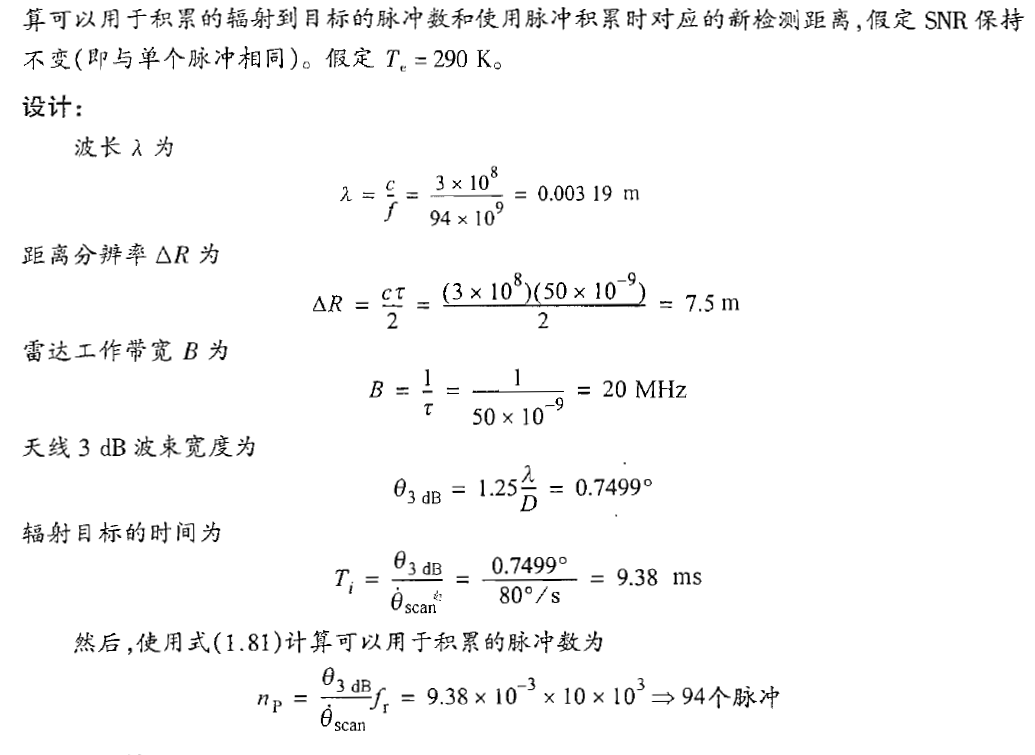
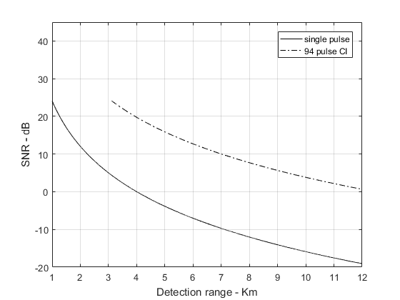
对应10dB时候的R_ref=2.245km

相关积累94个脉冲，SNR改善为19.73dB 是因为 SNR=10log10(94)

• 仿真代码

% Use this program to reproduce Fig. 1.19 and Fig. 120 of text.
close all
clear all
pt = 4; % peak power in Watts
freq = 94e+9; % radar operating frequency in Hz
g = 47.0; % antenna gain in dB
sigma = 20; % radar cross section in m squared
te = 290.0; % effective noise temperature in Kelvins
b = 20e+6; % radar operating bandwidth in Hz
nf = 7.0; %noise figure in dB
loss = 10.0; % radar losses in dB
range = linspace(1000,12000,10000); % range to target from 1. Km 12 Km, 1000 points
snr1 = radar_eq(pt, freq, g, sigma, te, b, nf, loss, range);
Rnewci=(94^0.25).*range;
snrCI=snr1+10*log10(94);%94 pulse coherent integration
%plot SNR versus range
figure(1)
rangekm  = range ./ 1000;
plot(rangekm,snr1,'k',Rnewci./1000,snr1,'k -.')
axis([1 12 -20 45])
grid
legend('single pulse','94 pulse CI')
xlabel ('Detection range - Km');
ylabel ('SNR - dB');

• 仿真实验图

SNR相对检测距离的曲线

 利用1.86式进行验证

• 仿真代码

% Use this program to reproduce Fig. 1.19 and Fig. 120 of text.
close all
clear all
pt = 4; % peak power in Watts
freq = 94e+9; % radar operating frequency in Hz
g = 47.0; % antenna gain in dB
sigma = 20; % radar cross section in m squared
te = 290.0; % effective noise temperature in Kelvins
b = 20e+6; % radar operating bandwidth in Hz
nf = 7.0; %noise figure in dB
loss = 10.0; % radar losses in dB
range = linspace(1000,12000,10000); % range to target from 1. Km 12 Km, 1000 points
snr1 = radar_eq(pt, freq, g, sigma, te, b, nf, loss, range);
Rnewci=(94^0.25).*range;
snrCI=snr1+10*log10(94);%94 pulse coherent integration
%plot SNR versus range
figure(1)
rangekm  = range ./ 1000;
plot(rangekm,snr1,'k',Rnewci./1000,snr1,'k -.')
axis([1 12 -20 45])
grid
legend('single pulse','94 pulse CI')
xlabel ('Detection range - Km');
ylabel ('SNR - dB');
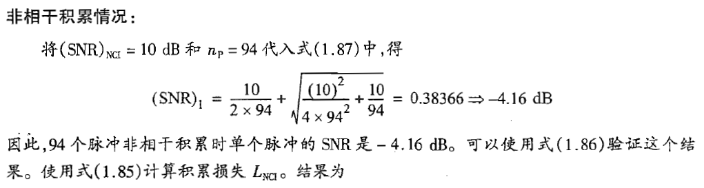
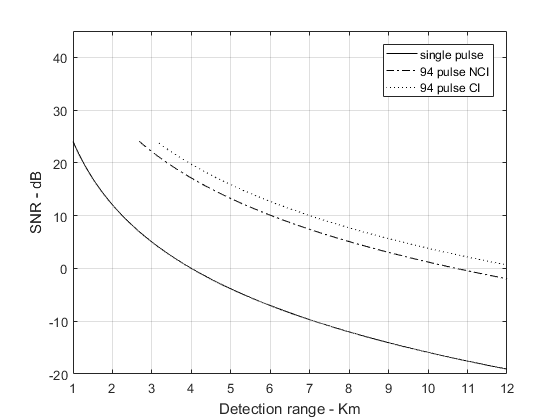
% Generate Figure 1.20
snr_b10 = 10.^(snr1./10);
SNR_1 = snr_b10./(2*94) + sqrt(((snr_b10.^2)./(4*94*94)) + (snr_b10./ 94)); % Equation 1.87 of text
LNCI = (1+SNR_1) / SNR_1; % Equation 1.78 of text
NCIgain = 10*log10(94) - 10*log10(LNCI);
Rnewnci = ((10.^(0.1*NCIgain)).^0.25).*range;
snrnci = snr1+NCIgain;
figure (2)
plot(rangekm,snr1,'k',Rnewnci./1000,snr1,'k -.', Rnewci./1000,snr1,'k:')
axis([1 12 -20 45])
grid
legend('single pulse','94 pulse NCI','94 pulse CI')
xlabel ('Detection range - Km');
ylabel ('SNR - dB');

• 仿真结果

SNR相对检测距离的曲线

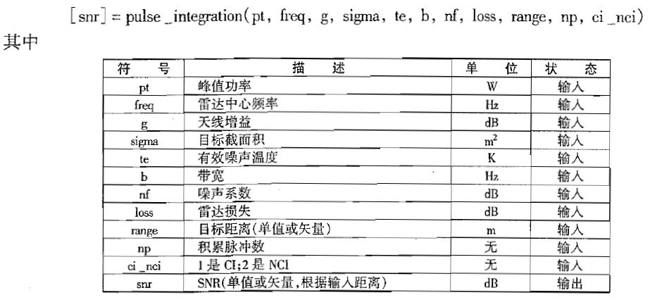
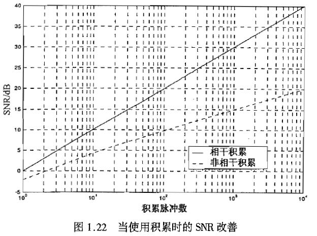
• SNR增益相对积累脉冲数的关系

下图1给出了SNR增益相对积累脉冲数的关系,其中包含相干积累和非相干积累两种情况。这幅图对应于前一个例题在R=5.01 km处的参数。图2给出了一般情况下SNR改善相对脉冲积累数的关系。

• [snrout] = pulse_integration(pt, freq, g, sigma, te, b, nf, loss, range,np,ci_nci)

function [snrout] = pulse_integration(pt, freq, g, sigma, te, b, nf, loss, range,np,ci_nci)
 snr1 = radar_eq(pt, freq, g, sigma, te, b, nf, loss, range) % single pulse SNR
if (ci_nci == 1) % coherent integration
   snrout = snr1 + 10*log10(np);
else % non-coherent integration
    if (ci_nci == 2)
        snr_nci = 10.^(snr1./10);
        val1 = (snr_nci.^2) ./ (4.*np.*np);
        val2 = snr_nci ./ np;
        val3 = snr_nci ./ (2.*np);
        SNR_1 = val3 + sqrt(val1 + val2); % Equation 1.87 of text
        LNCI = (1+SNR_1) ./ SNR_1; % Equation 1.85 of text
        snrout = snr1 + 10*log10(np) - 10*log10(LNCI);
    end
end
return

• R=5.01km对应的相干脉冲积累和非相干脉冲积累的仿真图

• 一般情况下