MATLAB-基本信号处理

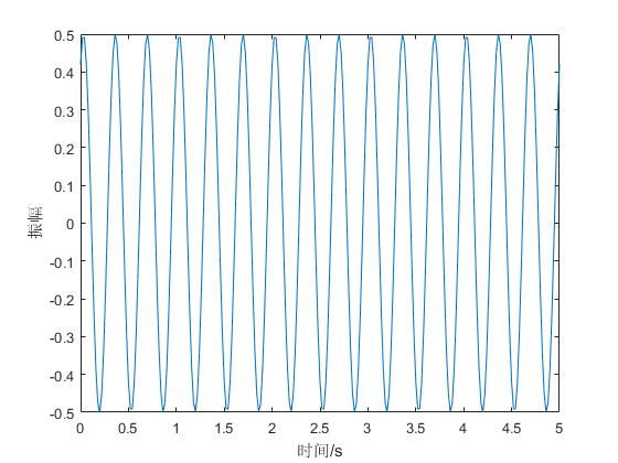
• 信号：频率为3Hz，采样间隔为0.02s的振动，振动振幅为0.5，初相为1，采样长度为5s

dt=0.02; %采样间隔
f=3; %采样频率
t=0:dt:5; %采样长度 振动持续时间
x=0.5*sin(2*pi*f*t+1); %信号
plot(t,x)
xlabel('时间/s')
ylabel('振幅')

• 信号同频率振动的结果：两个信号振动频率均为3Hz、采样间隔为0.02s的200个时间点的振动合成。
• 第一个振幅0.5 初相1 第二个振幅0.3 初相2.2

dt=0.02; %采样间隔
f1=3,f2=3; %采样频率
N=200;%采样点数
n=0:N-1;t=n*dt; %定义时间离散值
x1=0.5*sin(2*pi*f1*t+1); %信号1
x2=0.3*sin(2*pi*f2*t+2.2); %信号2
subplot(3,1,1),plot(t,x1);ylim([-1,1])
title('第一个信号')
xlabel('时间/s')
ylabel('振幅')
subplot(3,1,2),plot(t,x2);ylim([-1,1])
title('第二个信号')
xlabel('时间/s')
ylabel('振幅')
subplot(3,1,3),plot(t,x1+x2);ylim([-1,1])
title('合成信号')
xlabel('时间/s')
ylabel('振幅')

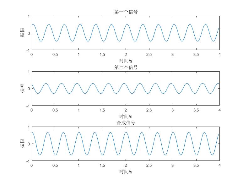
 发现两个频率相同的信号合成后的频率不变

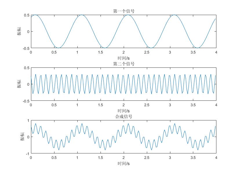
• 信号不同频率振动的结果：两个信号振动频率分别为1Hz和9Hz、振幅为0.5和0.3、初相为1和2.2，采样间隔为0.02s的200个时间点的振动合成。

dt=0.02; %采样间隔
f1=1,f2=9; %采样频率
N=200;%采样点数
n=0:N-1;t=n*dt; %定义时间离散值
x1=0.5*sin(2*pi*f1*t+1); %信号1
x2=0.3*sin(2*pi*f2*t+2.2); %信号2
subplot(3,1,1),plot(t,x1);
title('第一个信号')
xlabel('时间/s')
ylabel('振幅')
subplot(3,1,2),plot(t,x2);
title('第二个信号')
xlabel('时间/s')
ylabel('振幅')
subplot(3,1,3),plot(t,x1+x2);
title('合成信号')
xlabel('时间/s')
ylabel('振幅')

• 两个信号频率分别为10Hz和9Hz，振幅为0.3、初相位为1，采样间隔为0.01s，共400个时间点

dt=0.01; %采样间隔
f1=10,f2=9; %采样频率
N=400;%采样点数
n=0:N-1;t=n*dt; %定义时间离散值
x1=0.3*sin(2*pi*f1*t+1); %信号1
x2=0.3*sin(2*pi*f2*t+1); %信号2
subplot(3,1,1),plot(t,x1);
title('第一个信号')
xlabel('时间/s')
ylabel('振幅')
subplot(3,1,2),plot(t,x2);
title('第二个信号')
xlabel('时间/s')
ylabel('振幅')
subplot(3,1,3),plot(t,x1+x2);
title('合成信号')
xlabel('时间/s')
ylabel('振幅')

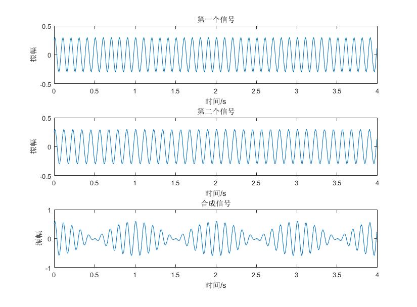
两个振幅相同，初相位也相同，而频率相差很小的两个简谐振动叠加时，就会产生非简谐振动：高频振动振幅包络线随时间而周期变换

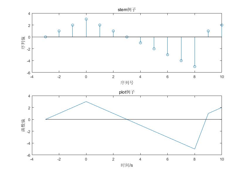
• 设一个信号值为{0 1 2 3 2 1 0 -1 -2 -3 -4 -5 1 2}，序号从-3到10。设信号的采样间隔为1s 用stem和plot函数表示这个信号

N=[-3 -2 -1 0 1 2 3 4 5 6 7 8 9 10]; %序号序列
X=[0 1 2 3 2 1 0 -1 -2 -3 -4 -5 1 2]; %值序列
subplot(2,1,1),stem(N,X); 
hold on;plot(N,zeros(1,length(X)),'k')%k表示黑色
%画出横轴
set(gca,'box','on'); %将坐标轴设在方框上
xlabel('序列号');
ylabel('序列值');
title('stem例子');
dt=1;t=N*dt;%给出时间间隔是时间序列
subplot(2,1,2),plot(t,X); 
hold on;plot(t,zeros(1,length(X)),'k')%k表示黑色
%画出横轴
xlabel('时间/s');
ylabel('函数值');
title('plot例子');

• 有一个振幅为1、频率为10Hz、相位为0.3的模拟信号，用0.01s的采样间隔（采样频率为100Hz）来表示原始信号
• 若采样变为0.1，画出原始信号和采样后的信号

dt=0.01;
t=0:dt:1;
f=10; %原始信号的频率为10Hz
x1=sin(2*pi*f*t+0.3);
dt1=0.1;
t1=0:dt1:1;
subplot(3,1,1),plot(t,x1),ylim([-1,1]);
title('原始信号')
xlabel('时间/s')
x2=sin(2*pi*f*t1+0.3);
subplot(3,1,2),plot(t1,x2),ylim([-1,1]);
title('采样后信号')
xlabel('时间/s')
subplot(3,1,3),plot(t,x1,t1,x2,'o'),ylim([-1,1])
title('采样过程')
xlabel('时间/s')

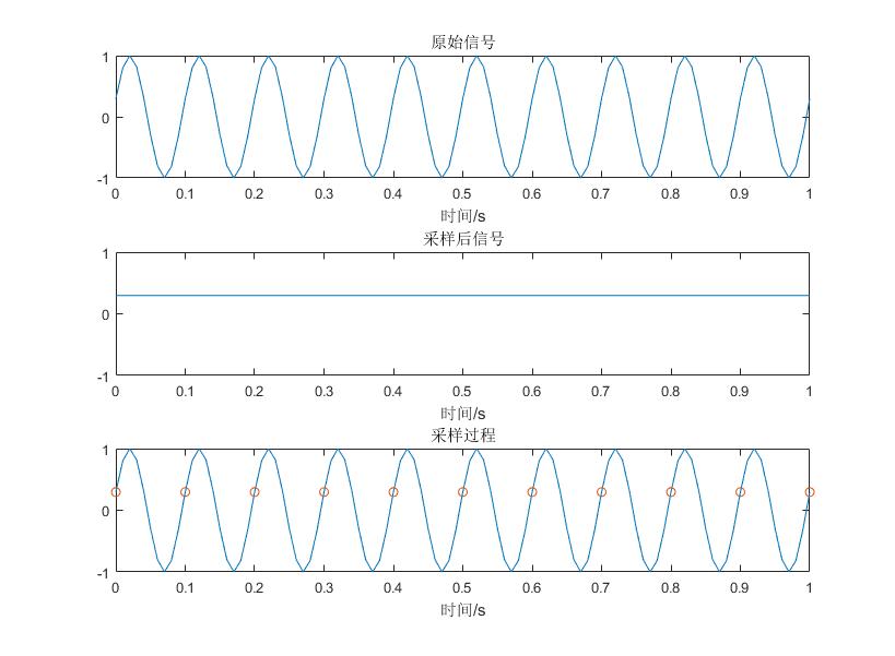
采样后的信号具有零频率的特征，是由采样过程造成的

• 把上述的频率改为9Hz 会出现假频的现象

dt=0.01;
t=0:dt:1;
f=9; %原始信号的频率为10Hz
x1=sin(2*pi*f*t+0.3);
dt1=0.1;
t1=0:dt1:1;
subplot(3,1,1),plot(t,x1),ylim([-1,1]);
title('原始信号')
xlabel('时间/s')
x2=sin(2*pi*f*t1+0.3);
subplot(3,1,2),plot(t1,x2),ylim([-1,1]);
title('采样后信号')
xlabel('时间/s')
subplot(3,1,3),plot(t,x1,t1,x2,'o'),ylim([-1,1])
title('采样过程')
xlabel('时间/s')

　　

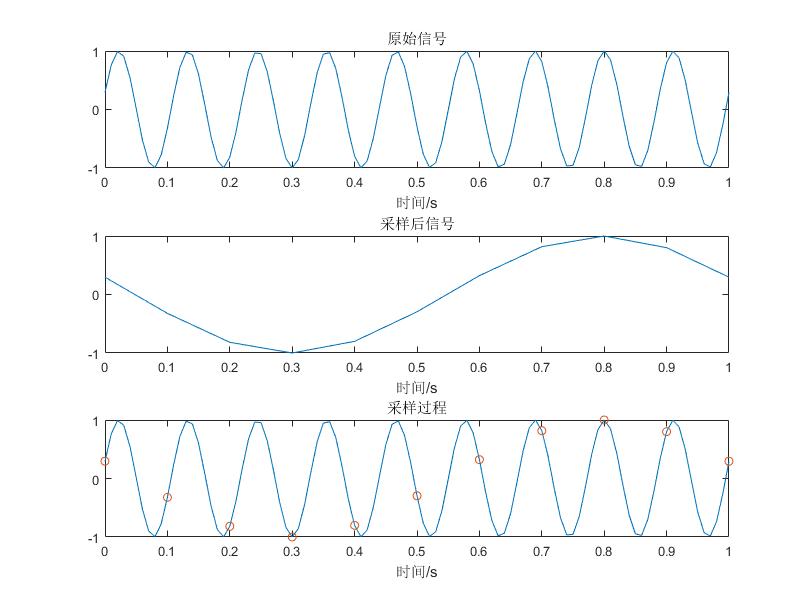
通过分析可以得到当采样频率大于信号中所含信号最大频率的两倍时，采样后的数据可以不失真地描述信号，当采样频率不满足这个条件时，会出现频率折叠和频率重复——>采样定理

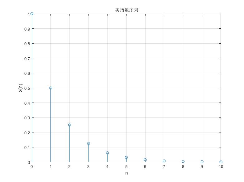
• 基本信号 1.指数信号x(n)=aⁿ
• 利用stem函数绘制0.5ⁿ，n从0到10

n=[0:10];
x=(0.5).^n;
stem(n,x)
xlabel('n'),ylabel('x(n)'),title('实指数序列');
grid on %添加网格线

• 正余弦信号f(t)=Ksin(wt+φ)；K为振幅，w为角频率，φ为初相位
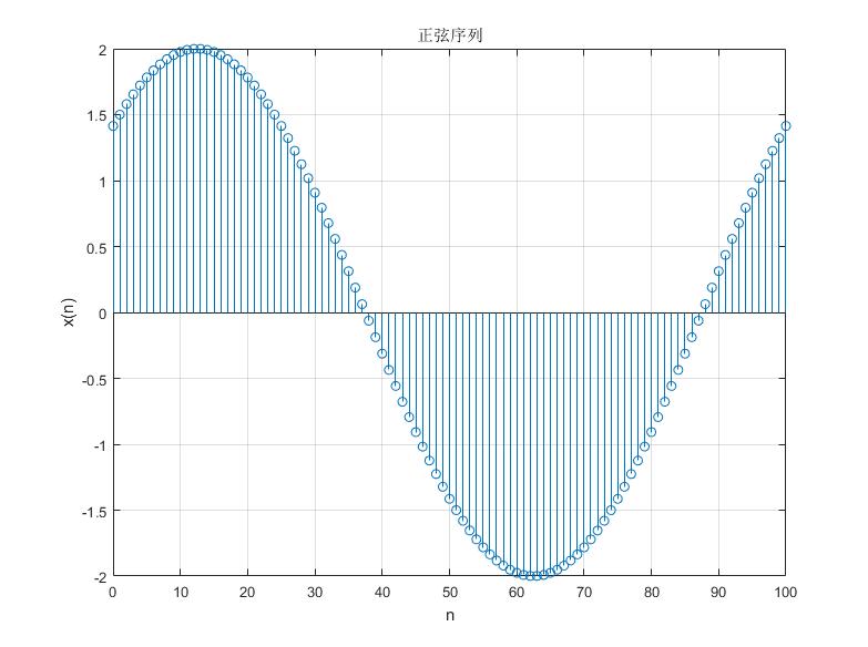
• 绘制x(n)=2sin(0.02*pi*n+pi/4)函数

n=[0:100];
x=2*sin(0.02*pi*n+pi/4);
stem(n,x)
xlabel('n'),ylabel('x(n)'),title('正弦序列');
grid on %添加网格线

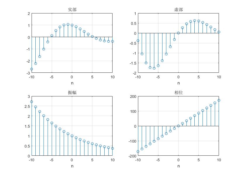
• 用-10~10的序号序列，绘制f(n)=e^(-0.1+j0.3)n的实部信号、虚部信号、振幅信号、相位信号

n=[-10:10];
alpha=-0.1+0.3*j;
x=exp(alpha*n);
Real_x=real(x);%实部
Image_x=imag(x);%虚部
Mag_x=abs(x);%z振幅
Phase_x=(180/pi)*angle(x);%相位 转化为度
subplot(2,2,1),stem(n,Real_x);
xlabel('n'),title('实部');grid on %添加网格线
subplot(2,2,2),stem(n,Image_x);
xlabel('n'),title('虚部');grid on %添加网格线
subplot(2,2,3),stem(n,Mag_x);
xlabel('n'),title('振幅');grid on %添加网格线
subplot(2,2,4),stem(n,Phase_x);
xlabel('n'),title('相位');grid on %添加网格线

• 随机信号 rand(1,n) 产生1行n列的在[0,1]上均匀分布的随机序列函数
• randn(1,n)产生1行n列均值为0，方差为1的高斯随机序列，即白噪声序列
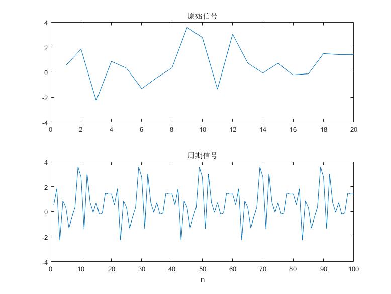
• 周期序列：将原始信号进行重复叠加

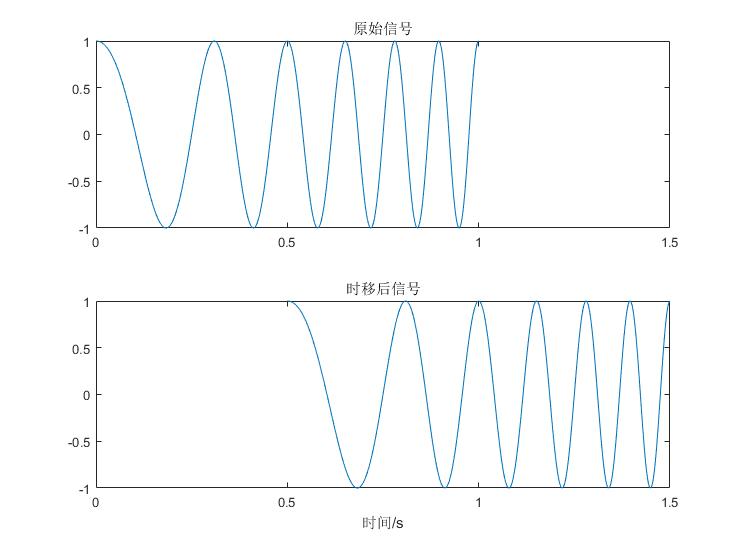
•  信号时移：产生一个从2Hz增加到10Hz的啁啾信号，并将其推迟500个采样间隔
• sigshift.m

function[y,n]=sigshift(x,m,n0)
%执行信号移位:y(n)=x(n+n0)
n=m+n0;y=x;

• 代码

t=0:0.001:1;%1s的时间段，以1kHz的采样频率采样
fo=2;f1=10;%信号从2Hz增加到10Hz
x=chirp(t,fo,1,f1);%在时间序列t上产生频率渐增的啁啾信号1表示在该时刻上频率变为f1
m=1:length(x);%m为信号的信号序列
subplot(2,1,1),plot((m-1)*0.001,x)%m为序号 m-1才与采样间隔相对应 
xlim([0 1.5]),title('原始信号')
[y,n]=sigshift(x,m,500);
subplot(2,1,2),plot((n-1)*0.001,y)
xlim([0 1.5]),title('时移后信号'),xlabel('时间/s')

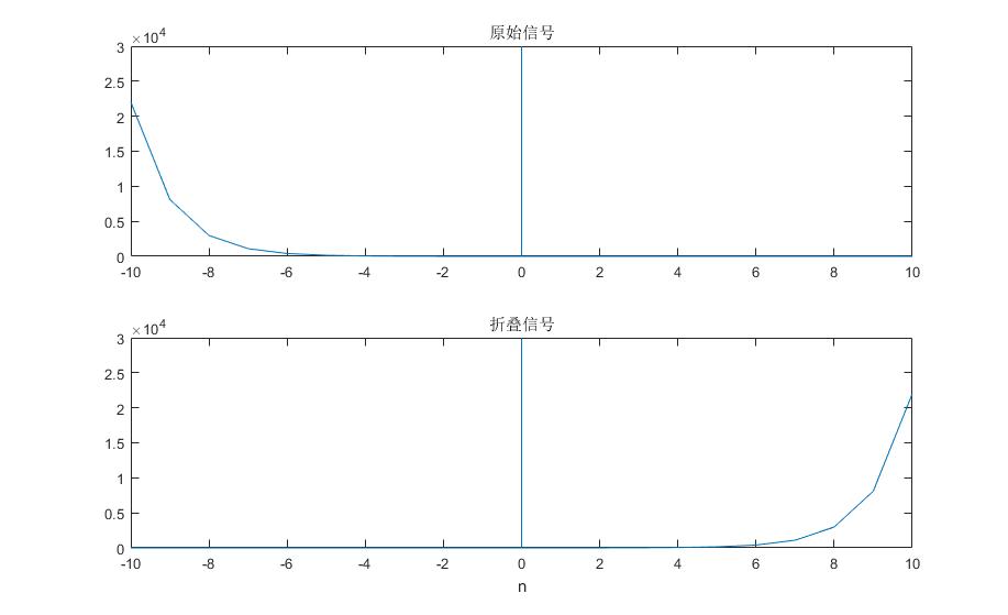
• 信号折叠
• 用-10~10的序号序列，给出离散序列e^(-n)的折叠信号
• sigfold.m

function [y,n]=sigfold(x,n)
  %执行信号折叠：y(n)=x(-n)
  y=fliplr(x);n=-fliplr(n);
  %fliplr函数的作用是对输入的序列进行左右翻转，若原来是[1,2,3,4],那之后是[4,3,2,1]
  

　　代码：

n=-10:10; %序列序号
x=exp(-n) %原始信号
subplot(2,1,1),plot(n,x),title('原始信号')
%绘制原始信号
line([0 0],ylim)%绘制一条坐标在0的直线
[y,n]=sigfold(x,n);%将x信号进行折叠
subplot(2,1,2),plot(n,y),title('折叠信号')
line([0 0],ylim)%绘制一条坐标在0的直线
xlabel('n')

 

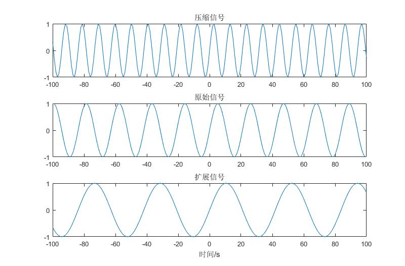
•  信号尺度变换：将-100到100的序列序号给出的正弦信号压缩扩展两倍，时间间隔为0.3s

%信号尺度变换
n=-100:100;%序号序列
dt=0.3;%时间间隔
t=n*dt;%时间序列
y=sin(t);%原始信号
y1=sin(2*t);
y2=sin(0.5*t);
subplot(3,1,1),plot(n,y1),title('压缩信号')
subplot(3,1,2),plot(n,y),title('原始信号')
subplot(3,1,3),plot(n,y2),title('扩展信号')
xlabel('时间/s')

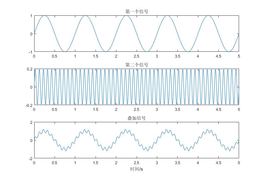
• 信号加：将频率1Hz和10Hz，振幅1和0.2的正弦信号叠加

dt=0.01;f1=1;f2=10;
n=0:500;
t=n*dt;
x1=sin(2*pi*f1*t);
x2=0.2*sin(2*pi*f2*t);
subplot(3,1,1),plot(t,x1),title('第一个信号')
subplot(3,1,2),plot(t,x2),title('第二个信号')
[y,n]=sigadd(x1,n,x2,n);
subplot(3,1,3),plot(t,y),title('叠加信号')
xlabel('时间/s')

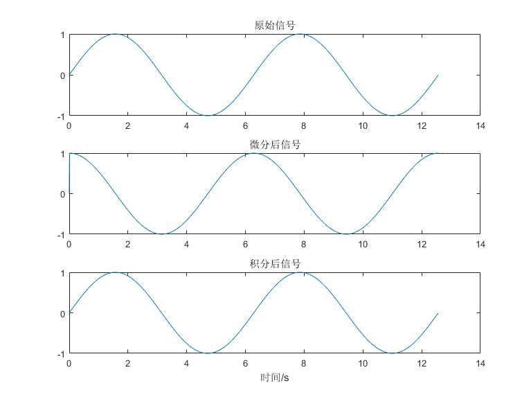
• 信号微分和积分

dt=0.01;
t=0:dt:4*pi;
y1=sin(t);
subplot(3,1,1),plot(t,y1),title('原始信号')
y2=diff(y1)/dt;%对信号进行微分
subplot(3,1,2),plot(t,[0 y2]),title('微分后信号')
%微分后的信号比原始信号少一个元素
for ii=1:length(y2)
    y3(ii)=sum(y2(1:ii))*dt;
end
subplot(3,1,3),plot(t,[0 y3]),title('积分后信号')
xlabel('时间/s')

• 信号乘
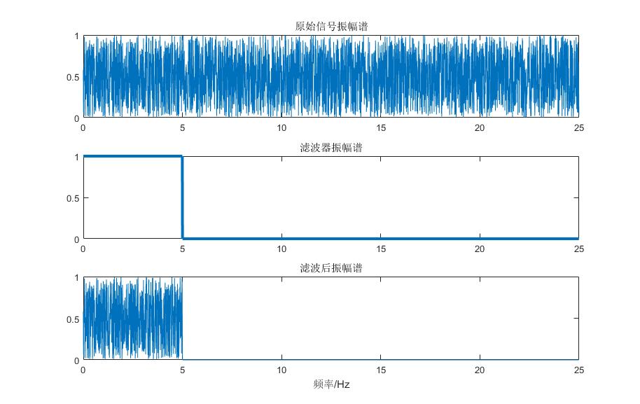
• 信号频率分辨率：分辨两个不同频率信号的最小间隔

 

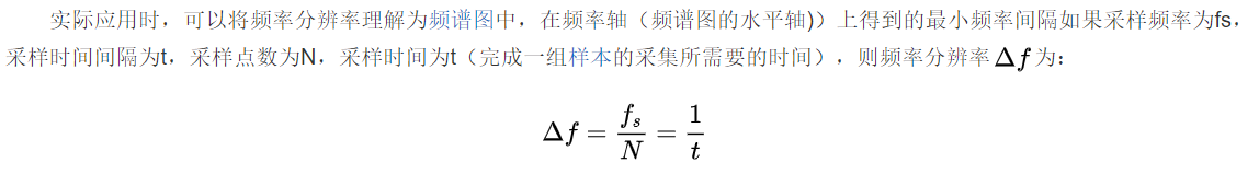
•  采样间隔为0.02s，采样频率为50Hz，长度为2min，信号具有6000个数据，则信号频率分辨率为df=1/(6000*dt)，在频率域中去除5Hz以上的高频信号
• sigmult.m

function[y,n]=sigmult(x1,n1,x2,n2)
%执行信号相乘 y(n)=x1(n)*x2(n)
%x1是第一个信号 序列号为n1
%x2是第二个信号 序列号为n2
%n1和n2可以不同
n=min(min(n1),min(n2)):max(max(n1),max(n2));
%得到y(n)的信号序列的序列号
y1=zeros(1,length(n));y2=y1;%初始化信号
y1(find(n>=min(n1))&(n<=max(n1))==1)=x1;
y2(find(n>=min(n2))&(n<=max(n2))==1)=x2;
y=y1.*y2;

代码：

dt=0.02;
df=1/(6000*dt);
%信号长度为2分钟的频率分辨率
%分辨两个不同频率信号的最小间隔
n=0:2999;%取前3000个信号进行操作
f=n*df;
sig=rand(1,length(n));%运用随机函数产生信号振幅谱
filt=[ones(1,5/df),zeros(1,(length(n)-5/df))];
subplot(3,1,1),plot(f,sig),title('原始信号振幅谱')
[y,n1]=sigmult(filt,n,sig,n);
subplot(3,1,2),plot(f,filt,'LineWidth',3),title('滤波器振幅谱')
subplot(3,1,3),plot(f,y),title('滤波后振幅谱')
xlabel('频率/Hz')

• 第3章 Fourier变换