PyTorch-神经网络
- anaconda镜像网站
https://mirrors.bfsu.edu.cn/anaconda/archive/
- 使用Pytorch tensors来创建前向神经网络,计算损失,以及反向传播
- 一个Pytorch Tensor很像一个numpy的ndarray。但它和numpy ndarray最大的区别是,Pytorch Tensor可以在CPU或者GPU上运算
- 如果想在GPU上计算,就需要把Tensor换成cuda类型。
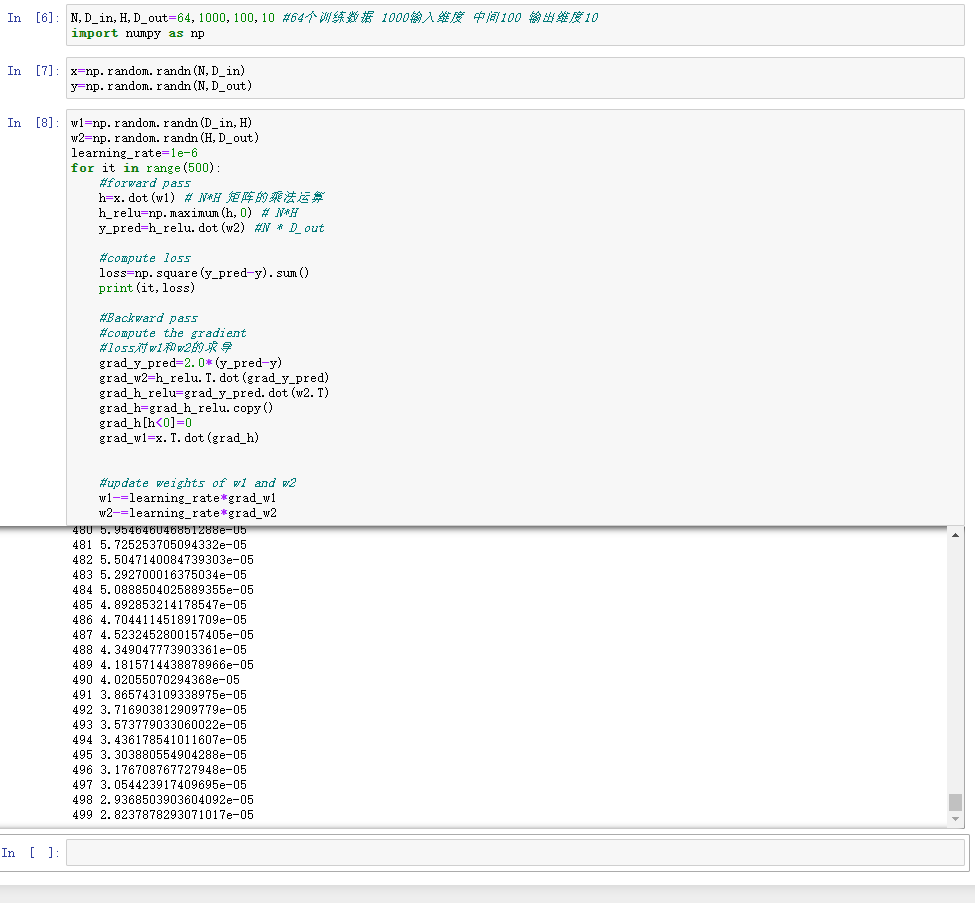
N,D_in,H,D_out=64,1000,100,10 #64个训练数据 1000输入维度 中间100 输出维度10
import numpy as np
x=np.random.randn(N,D_in)
y=np.random.randn(N,D_out)
w1=np.random.randn(D_in,H)
w2=np.random.randn(H,D_out)
learning_rate=1e-6
for it in range(500):
    #forward pass
    h=x.dot(w1) # N*H 矩阵的乘法运算
    h_relu=np.maximum(h,0) # N*H
    y_pred=h_relu.dot(w2) #N * D_out

    #compute loss
    loss=np.square(y_pred-y).sum()
    print(it,loss)

    #Backward pass
    #compute the gradient
    #loss对w1和w2的求导
    grad_y_pred=2.0*(y_pred-y)
    grad_w2=h_relu.T.dot(grad_y_pred)
    grad_h_relu=grad_y_pred.dot(w2.T)
    grad_h=grad_h_relu.copy()
    grad_h[h<0]=0
    grad_w1=x.T.dot(grad_h)


    #update weights of w1 and w2
    w1-=learning_rate*grad_w1
    w2-=learning_rate*grad_w2
- 若出现导入torch失败的情况 就点击

然后输出
pip install torch
- 利用torch版本进行训练
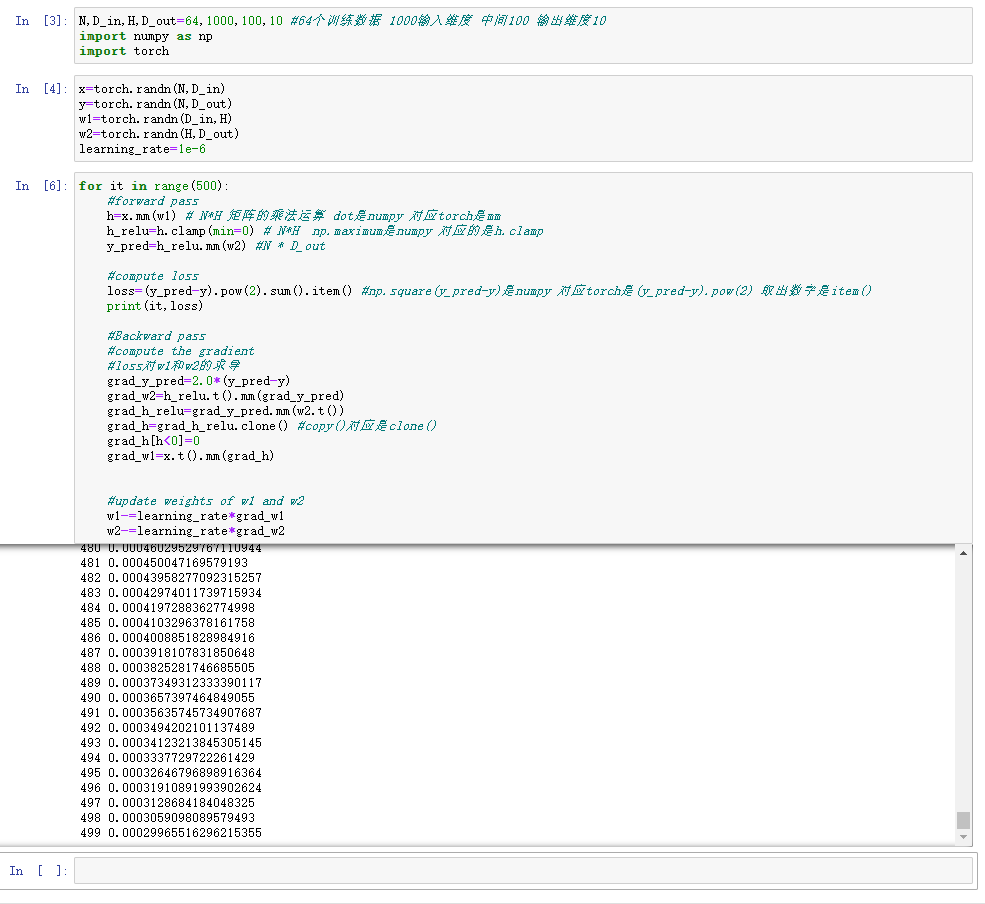
N,D_in,H,D_out=64,1000,100,10 #64个训练数据 1000输入维度 中间100 输出维度10
import numpy as np
import torch
x=torch.randn(N,D_in)
y=torch.randn(N,D_out)
w1=torch.randn(D_in,H)
w2=torch.randn(H,D_out)
learning_rate=1e-6
for it in range(500):
    #forward pass
    h=x.mm(w1) # N*H 矩阵的乘法运算 dot是numpy 对应torch是mm
    h_relu=h.clamp(min=0) # N*H  np.maximum是numpy 对应的是h.clamp
    y_pred=h_relu.mm(w2) #N * D_out

    #compute loss
    loss=(y_pred-y).pow(2).sum().item() #np.square(y_pred-y)是numpy 对应torch是(y_pred-y).pow(2) 取出数字是item()
    print(it,loss)

    #Backward pass
    #compute the gradient
    #loss对w1和w2的求导
    grad_y_pred=2.0*(y_pred-y)
    grad_w2=h_relu.t().mm(grad_y_pred)
    grad_h_relu=grad_y_pred.mm(w2.t())
    grad_h=grad_h_relu.clone() #copy()对应是clone()
    grad_h[h<0]=0
    grad_w1=x.t().mm(grad_h)


    #update weights of w1 and w2
    w1-=learning_rate*grad_w1
    w2-=learning_rate*grad_w2
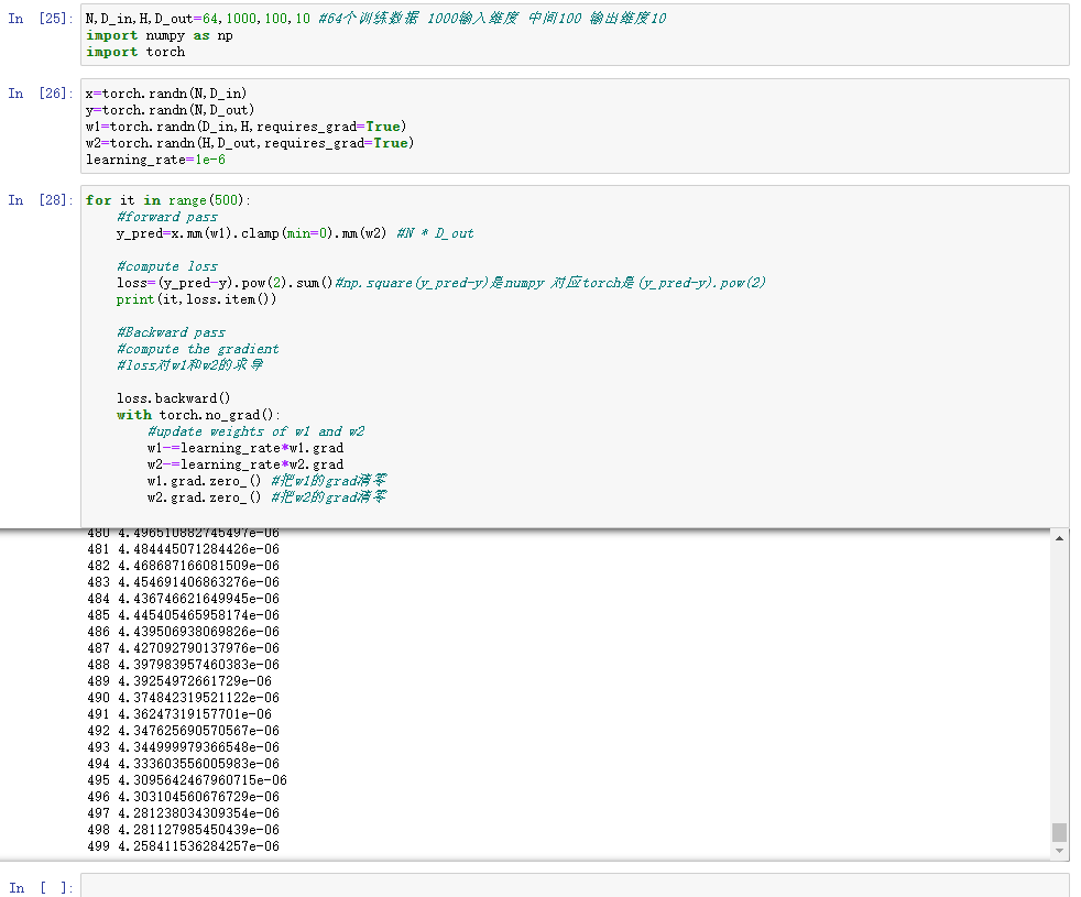
- pytorch可以自动计算梯度值
x=torch.tensor(1.,requires_grad=True)
w=torch.tensor(2.,requires_grad=True)
b=torch.tensor(3.,requires_grad=True)

y=w*x+b
y.backward()

#dy/dx=w
print(w.grad)
print(x.grad)
print(b.grad)

- 利用pytorch可以自动计算梯度值,来构建前向神经网络
N,D_in,H,D_out=64,1000,100,10 #64个训练数据 1000输入维度 中间100 输出维度10
import numpy as np
import torch
x=torch.randn(N,D_in)
y=torch.randn(N,D_out)
w1=torch.randn(D_in,H,requires_grad=True)
w2=torch.randn(H,D_out,requires_grad=True)
learning_rate=1e-6
for it in range(500):
    #forward pass
    y_pred=x.mm(w1).clamp(min=0).mm(w2) #N * D_out

    #compute loss
    loss=(y_pred-y).pow(2).sum()#np.square(y_pred-y)是numpy 对应torch是(y_pred-y).pow(2)
    print(it,loss.item())

    #Backward pass
    #compute the gradient
    #loss对w1和w2的求导

    loss.backward()
    with torch.no_grad():
        #update weights of w1 and w2
        w1-=learning_rate*w1.grad
        w2-=learning_rate*w2.grad
        w1.grad.zero_() #把w1的grad清零
        w2.grad.zero_() #把w2的grad清零
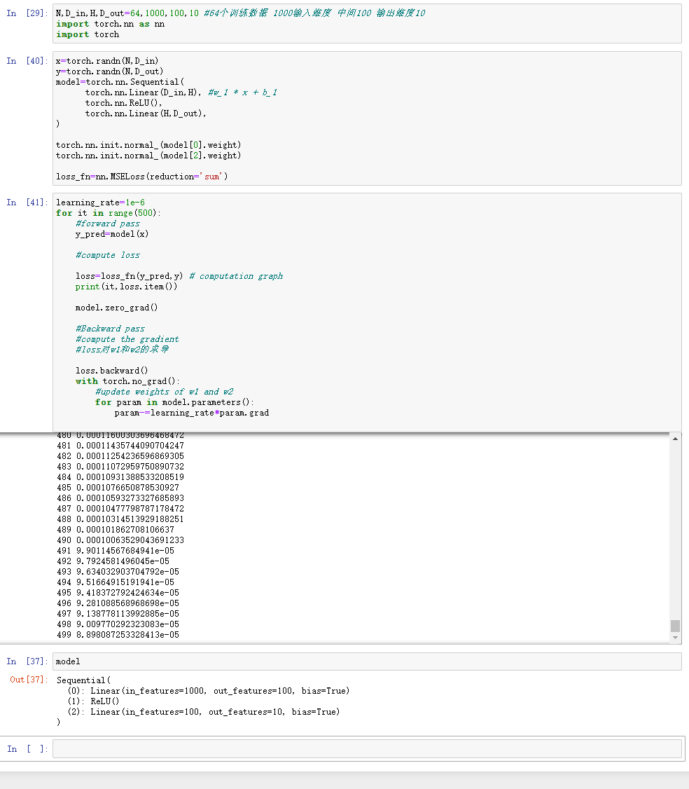
- 使用Pytorch中nn这个库来构建网络,用Pytorch autograd来构建计算图和计算gradients
N,D_in,H,D_out=64,1000,100,10 #64个训练数据 1000输入维度 中间100 输出维度10
import torch.nn as nn
import torch
x=torch.randn(N,D_in)
y=torch.randn(N,D_out)
model=torch.nn.Sequential(
      torch.nn.Linear(D_in,H), #w_1 * x + b_1
      torch.nn.ReLU(),
      torch.nn.Linear(H,D_out),
)

torch.nn.init.normal_(model[0].weight)
torch.nn.init.normal_(model[2].weight)

loss_fn=nn.MSELoss(reduction='sum')
learning_rate=1e-6
for it in range(500):
    #forward pass
    y_pred=model(x)

    #compute loss

    loss=loss_fn(y_pred,y) # computation graph
    print(it,loss.item())

    model.zero_grad()

    #Backward pass
    #compute the gradient
    #loss对w1和w2的求导

    loss.backward()
    with torch.no_grad():
        #update weights of w1 and w2
        for param in model.parameters():
            param-=learning_rate*param.grad
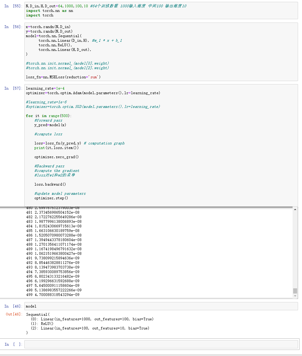
- Pytorch:optim
- 这一次我们不再手动更新模型的weight,而是使用optim这个包来帮助我们更新参数。optim这个package提供了各种不同的模型优化的方法
- 包括SGD-momentum、RMSProp、Adam等等
N,D_in,H,D_out=64,1000,100,10 #64个训练数据 1000输入维度 中间100 输出维度10
import torch.nn as nn
import torch
x=torch.randn(N,D_in)
y=torch.randn(N,D_out)
model=torch.nn.Sequential(
      torch.nn.Linear(D_in,H), #w_1 * x + b_1
      torch.nn.ReLU(),
      torch.nn.Linear(H,D_out),
)

#torch.nn.init.normal_(model[0].weight)
#torch.nn.init.normal_(model[2].weight)

loss_fn=nn.MSELoss(reduction='sum')
learning_rate=1e-4
optimizer=torch.optim.Adam(model.parameters(),lr=learning_rate)

#learning_rate=1e-6
#optimizer=torch.optim.SGD(model.parameters(),lr=learning_rate)

for it in range(500):
    #forward pass
    y_pred=model(x)

    #compute loss

    loss=loss_fn(y_pred,y) # computation graph
    print(it,loss.item())

    optimizer.zero_grad()

    #Backward pass
    #compute the gradient
    #loss对w1和w2的求导

    loss.backward()

    #update model parameters
    optimizer.step()
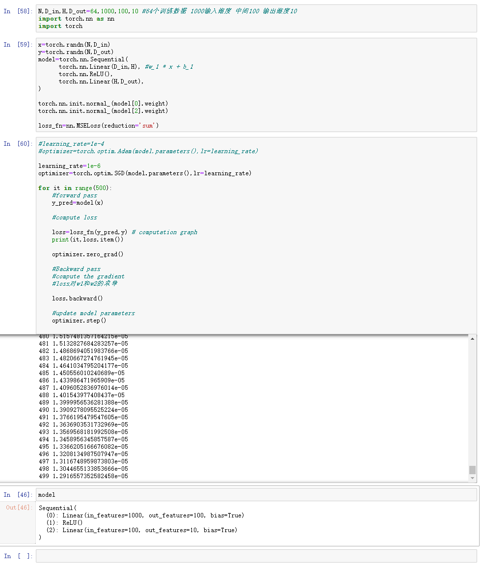
- 不同的优化器,可能进行不同的调参 比如使用optim.SGD时候 需要加上
torch.nn.init.normal_(model[0].weight)
torch.nn.init.normal_(model[2].weight)
- 而使用optim.Adam则不需要
- optim.SGD代码如下:
N,D_in,H,D_out=64,1000,100,10 #64个训练数据 1000输入维度 中间100 输出维度10
import torch.nn as nn
import torch
x=torch.randn(N,D_in)
y=torch.randn(N,D_out)
model=torch.nn.Sequential(
      torch.nn.Linear(D_in,H), #w_1 * x + b_1
      torch.nn.ReLU(),
      torch.nn.Linear(H,D_out),
)

torch.nn.init.normal_(model[0].weight)
torch.nn.init.normal_(model[2].weight)

loss_fn=nn.MSELoss(reduction='sum')
#learning_rate=1e-4
#optimizer=torch.optim.Adam(model.parameters(),lr=learning_rate)

learning_rate=1e-6
optimizer=torch.optim.SGD(model.parameters(),lr=learning_rate)

for it in range(500):
    #forward pass
    y_pred=model(x)

    #compute loss

    loss=loss_fn(y_pred,y) # computation graph
    print(it,loss.item())

    optimizer.zero_grad()

    #Backward pass
    #compute the gradient
    #loss对w1和w2的求导

    loss.backward()

    #update model parameters
    optimizer.step()
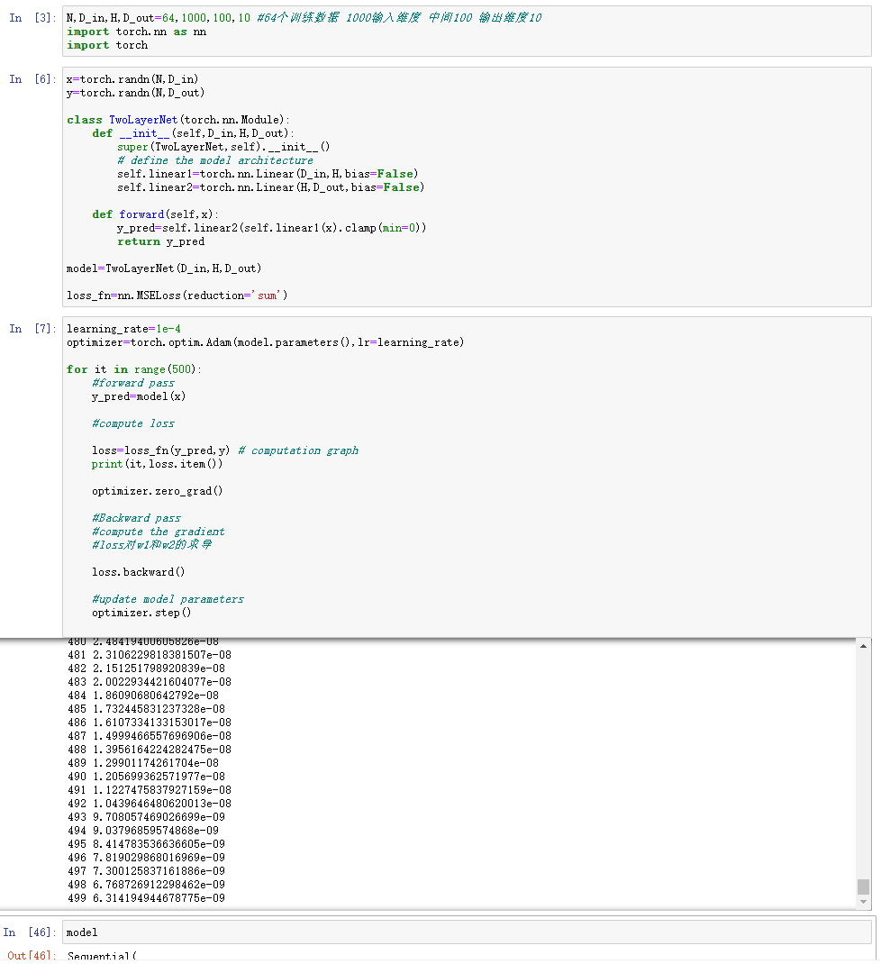
- Pytorch:自定义nn Modules
- 定义一个模型,这个模型继承自nn.Module类。如果需要定义一个比Sequential模型更加复杂的模型,就需要定义nn.Module模型
N,D_in,H,D_out=64,1000,100,10 #64个训练数据 1000输入维度 中间100 输出维度10
import torch.nn as nn
import torch
x=torch.randn(N,D_in)
y=torch.randn(N,D_out)

class TwoLayerNet(torch.nn.Module):
    def __init__(self,D_in,H,D_out):
        super(TwoLayerNet,self).__init__()
        # define the model architecture
        self.linear1=torch.nn.Linear(D_in,H,bias=False)
        self.linear2=torch.nn.Linear(H,D_out,bias=False)

    def forward(self,x):
        y_pred=self.linear2(self.linear1(x).clamp(min=0))
        return y_pred

model=TwoLayerNet(D_in,H,D_out)

loss_fn=nn.MSELoss(reduction='sum')
learning_rate=1e-4
optimizer=torch.optim.Adam(model.parameters(),lr=learning_rate)

for it in range(500):
    #forward pass
    y_pred=model(x)

    #compute loss

    loss=loss_fn(y_pred,y) # computation graph
    print(it,loss.item())

    optimizer.zero_grad()

    #Backward pass
    #compute the gradient
    #loss对w1和w2的求导

    loss.backward()

    #update model parameters
    optimizer.step()
转载请注明出处,欢迎讨论和交流!