深度学习—LeNet5_CIFAR100代码

 

 

 

 

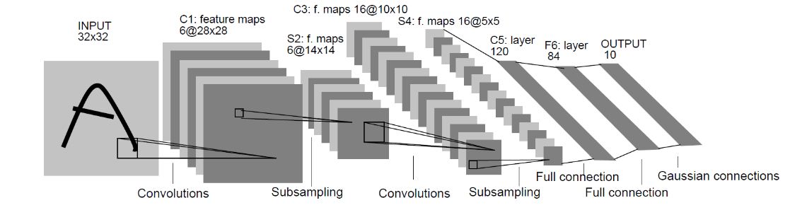
import torch
from torch.utils.data import DataLoader
from torchvision import transforms
from torchvision import datasets

##########################################################
# ==> 1.准备数据
##########################################################
# 预处理
transfrom = transforms.Compose([
    transforms.ToTensor()
])
# 准备训练集数据和验证集
train_transfrom= transforms.Compose([
    # 此处可以添加你所用到的数据增强方法
    transforms.RandomHorizontalFlip(p=0.5),
    transforms.ToTensor()
])
train_dataset = datasets.CIFAR100(root='你的路径',transform=train_transfrom,train=True,download=True)#注意在训练集中添加数据增强方法
val_dataset = datasets.CIFAR100(root='你的路径',transform=transfrom,train=False,download=True)

# 训练集dataloader，验证集dataloader
train_loader = DataLoader(
    dataset=train_dataset,
    batch_size=128,
    shuffle=True
)
val_loader = DataLoader(
    dataset=val_dataset,
    batch_size=128,
    shuffle=False
)
##########################################################
# ==> 2.搭建网络
##########################################################
# 重写nn.Module类，使用自己的网络
from torch import nn
# 此处可以在网络中添加一些卷积层（或其他层）
from torch import nn
# 定义LeNet-5网络
class My_Net(nn.Module):
    def __init__(self):
        super(My_Net, self).__init__()
        # 输入3×32×32的CIFAR-100图像，经过卷积后输出大小为6×28×28
        self.conv1 = nn.Conv2d(in_channels=3,
                               out_channels=6,
                               kernel_size=(5, 5),
                               stride=1,
                               bias=True)
        # 卷积操作后使用Tanh激活函数,激活函数不改变其大小
        self.tanh1 = nn.Tanh()
        # 使用最大池化进行下采样，输出大小为6×14×14
        self.pool1 = nn.MaxPool2d(kernel_size=(2, 2),
                                  stride=2)
        # 输出大小为16×10×10
        self.conv2 = nn.Conv2d(in_channels=6,
                               out_channels=16,
                               kernel_size=(5, 5),
                               stride=1,
                               bias=True)
        self.tanh2 = nn.Tanh()
        # 输出大小为16×5×5
        self.pool2 = nn.MaxPool2d(kernel_size=(2, 2),
                                  stride=2)
        # 两个卷积层和最大池化层后接三个全连接层
        self.fc1 = nn.Linear(16*5*5, 120)
        self.tanh3 = nn.Tanh()
        self.fc2 = nn.Linear(120, 84)
        self.tanh4 = nn.Tanh()
        # 第三个全连接层是输出层，输出单元个数即是数据集中类的个数，CIFAR-100数据集有100个类
        self.classifier = nn.Linear(84, 100)

    # 定义前向传播过程
    def forward(self, x):
        x = self.conv1(x)
        x = self.tanh1(x)
        x = self.pool1(x)
        x = self.conv2(x)
        x = self.tanh2(x)
        x = self.pool2(x)
        # 在全连接操作前将数据平展开
        x = x.view(x.size(0), -1)
        x = self.fc1(x)
        x = self.tanh3(x)
        x = self.fc2(x)
        x = self.tanh4(x)
        output = self.classifier(x)
        return output
# 将网络类实例化，变成对象

# 定义训练的设备
device = torch.device('cuda:0' if torch.cuda.is_available() else 'cpu')
net = My_Net()
net = net.to(device)
##########################################################
# ==> 3.定义损失函数,优化器，学习率调整方式
##########################################################
# 3.1损失函数
loss_fn = nn.CrossEntropyLoss() # 使用CE Loss
loss_fn = loss_fn.to(device)
# 3.2优化器，学习率调整器
from torch import optim
# 使用SGD优化器，初始学习率为0.1
optimizer = optim.SGD(net.parameters(), lr=0.1)
# 使用StepLR学习率调整方式，每隔5个Epoch学习率变为原来的0.1倍
scheduler = optim.lr_scheduler.StepLR(optimizer, step_size=10, gamma=0.1)

##########################################################
# ==> 4.进行训练
##########################################################
# 迭代训练20个Epoch
num_epochs = 50
print("Start Train!")
for epoch in range(1, num_epochs+1):
    train_loss = 0
    train_acc = 0
    val_loss = 0
    val_acc = 0
    # 训练阶段，设为训练状态
    net.train()
    train_confusion_matrix = torch.zeros(100, 100).cuda()  # 训练集混淆矩阵
    val_confusion_matrix = torch.zeros(100, 100).cuda()  # 验证集混淆矩阵
    for batch_index, (imgs,labels) in enumerate(train_loader):
        imgs,labels = imgs.to(device),labels.to(device)
        output = net(imgs)
        loss = loss_fn(output,labels) #计算损失
        optimizer.zero_grad()# 梯度清零
        loss.backward()# 反向传播
        optimizer.step()# 梯度更新
        # 计算精确度
        _,predict = torch.max(output,dim=1)
        corec = (predict == labels).sum().item()
        acc = corec / imgs.shape[0]
        train_loss += loss.item()
        train_acc += acc

        for t, p in zip(labels.view(-1), output.argmax(dim=1).view(-1)):
            train_confusion_matrix[t.long(), p.long()] += 1

    # 查看训练集每个类的准确率
    acc_per_class = train_confusion_matrix.diag() / train_confusion_matrix.sum(1)
    acc_per_class = acc_per_class.cpu().numpy()
    print()
    print('train acc_per_class:\n',acc_per_class)
    # 验证阶段
    net.eval()
    for batch_index, (imgs, labels) in enumerate(val_loader):
        imgs, labels = imgs.to(device), labels.to(device)
        output = net(imgs)
        loss = loss_fn(output,labels)
        _, predict = torch.max(output, dim=1)
        corec = (predict == labels).sum().item()
        acc = corec / imgs.shape[0]
        val_loss += loss.item()
        val_acc += acc
        for t, p in zip(labels.view(-1), output.argmax(dim=1).view(-1)):
            val_confusion_matrix[t.long(), p.long()] += 1

    # 查看验证集每个类的准确率
    acc_per_class = val_confusion_matrix.diag() / val_confusion_matrix.sum(1)
    acc_per_class = acc_per_class.cpu().numpy()
    print()
    print('val acc_per_class:\n',acc_per_class)
    scheduler.step()
    # 依次输出当前epoch、总的num_epochs，
    # 训练过程中当前epoch的训练损失、训练精确度、验证损失、验证精确度和学习率
    print()
    print(epoch, '/', num_epochs,
          train_acc/len(train_loader),
          train_loss/len(train_loader),
          val_acc / len(val_loader),
          val_loss/len(val_loader),
         optimizer.param_groups[0]['lr'])

 

知识产权声明: 本博文中的ppt素材及相关内容和知识产权，均属于河南大学张重生老师所讲授的《深度学习》课程及张重生老师在2025年出版的著作《新一代人工智能 从深度学习到大模型》（机械工业出版社）。特此声明。

真挚地感谢张重生老师在本人于河南大学学习期间的教导。