[Scikit-learn] 2.3 Clustering - Spectral clustering
From: 2.3.5 Clustering - Spectral clustering
From: 漫谈 Clustering (4): Spectral Clustering
From: 漫谈 Clustering (番外篇): Dimensionality Reduction
传统方式的弊端
事实上,Laplacian Eigenmap (拉普拉斯特征映射) 假设数据分布在一个嵌套在高维空间中的低维流形上, Laplacian Matrix  则是流形的 Laplace Beltrami operator 的一个离散近似。关于流形以及 Laplacian Eigenmap 这个模型的理论知识就不在这里做更多地展开了,下面看一个比较直观的例子 Swiss Roll 。
Swiss Roll 是一个像面包圈一样的结构,可以看作一个嵌套在三维空间中的二维流形,如下图所示,左边是 Swiss Roll ,右边是从 Swiss Roll 中随机选出来的一些点,为了标明点在流形上的位置,给它们都标上了颜色。

【显然,这个东西没法用传统方式做聚类分析,直观的看上去,除了距离,还应该考虑结构因素】
而下图是 Laplacian Eigenmap 和 PCA 分别对 Swiss Roll 降维的结果,可以看到 LE 成功地把这个流形展开把在流形上属于不同位置的点映射到了不同的地方,而 PCA 的结果则很糟糕,几种颜色都混杂在了一起。

所以,Spectral Clustering便登场了!

可以看到,只有三个比较人性化:SpectralClustering, AgglomerativeClustering, DBSCAN
SpectralClustering
- 根据数据构造一个 Graph ,Graph 的每一个节点对应一个数据点,将相似的点连接起来,并且边的权重用于表示数据之间的相似度。把这个 Graph 用邻接矩阵的形式表示出来,记为
 。一个最偷懒的办法就是:直接用我们前面在 K-medoids 中用的相似度矩阵作为 。
 - 把 的每一列元素加起来得到
 个数,把它们放在对角线上(其他地方都是零),组成一个
  的矩阵,记为
  。并令
。并令  。
。 - 求出 的前
 个特征值(在本文中,除非特殊说明,否则“前 个”指按照特征值的大小从小到大的顺序)
 以及对应的特征向量
  。
。 - 把这 个特征(列)向量排列在一起组成一个
 的矩阵,将其中每一行看作 维空间中的一个向量,并使用 K-means 算法进行聚类。聚类的结果中每一行所属的类别就是原来 Graph 中的节点亦即最初的 个数据点分别所属的类别。
其实,如果你熟悉 Dimensional Reduction (降维)的话,大概已经看出来了,Spectral Clustering 其实就是:
通过 Laplacian Eigenmap 的降维方式降维之后再做 K-means 的一个过程。
不过,为什么要刚好降到 维呢?其实整个模型还可以从另一个角度导出来,所以,让我们不妨先跑一下题。
在 Image Processing (我好像之前有听说我对这个领域深恶痛绝?)里有一个问题就是对图像进行 Segmentation (区域分割),也就是让相似的像素组成一个区域,比如,我们一般希望一张照片里面的人(前景)和背景被分割到不同的区域中。在 Image Processing 领域里已经有许多自动或半自动的算法来解决这个问题,并且有不少方法和 Clustering 有密切联系。比如我们在谈 Vector Quantization 的时候就曾经用 K-means 来把颜色相似的像素聚类到一起,不过那还不是真正的 Segmentation ,因为如果仅仅是考虑颜色相似的话,图片上位置离得很远的像素也有可能被聚到同一类中,我们通常并不会把这样一些“游离”的像素构成的东西称为一个“区域”,但这个问题其实也很好解决:只要在聚类用的 feature 中加入位置信息(例如,原来是使用 R、G、B 三个值来表示一个像素,现在加入 x、y 两个新的值)即可。
Ref: http://blog.csdn.net/abcjennifer/article/details/8170687
将边权赋值为两点之间的similarity,做聚类的目标就是最小化类间connection的weight。

比如对于下面这幅图,分割如下

但是这样有可能会有问题,比如:

由于Graph cut criteria 只考虑了类间差小,而没考虑internal cluster density.所以会有上面分割的问题。这里引入Normalised-cut(Shi & Malik, 97')。
Graph Cut
另一方面,还有一个经常被研究的问题就是 Graph Cut ,简单地说就是把一个 Graph 的一些边切断,让他被打散成一些独立联通的 sub-Graph ,而这些被切断的边的权值的总和就被称为 Cut 值。
如果用一张图片中的所有像素来组成一个 Graph ,并把(比如,颜色和位置上)相似的节点连接起来,边上的权值表示相似程度,那么把图片分割为几个区域的问题实际上等价于把 Graph 分割为几个 sub-Graph 的问题,并且我们可以要求分割所得的 Cut 值最小,亦即:那些被切断的边的权值之和最小,直观上我们可以知道,权重比较大的边没有被切断,表示比较相似的点被保留在了同一个 sub-Graph 中,而彼此之间联系不大的点则被分割开来。我们可以认为这样一种分割方式是比较好的。
实际上,抛开图像分割的问题不谈,在 Graph Cut 相关的一系列问题中,Minimum cut (最小割)本身就是一个被广泛研究的问题,并且有成熟的算法来求解。只是单纯的最小割在这里通常并不是特别适用,很多时候只是简单地把和其他像素联系最弱的那一个像素给分割出去了,相反,我们通常更希望分割出来的区域(的大小)要相对均匀一些,而不是一些很大的区块和一些几乎是孤立的点。为此,又有许多替代的算法提出来,如 Ratio Cut 、Normalized Cut 等。
Laplacian Eigenmap
From: http://www.cnblogs.com/lmsj918/p/4075228.html
主要内容是Laplacian Eigenmap中的核心推导过程。

有空还是多点向这位师兄请教,每次都会捡到不少金子。
Reference : 《Laplacian Eigenmaps for Dimensionality Reduction and Data Representation》,2003,MIT
From: Spectral clustering for image segmentation
我非常喜欢的一个示例代码
print(__doc__)
# Authors: Emmanuelle Gouillart <emmanuelle.gouillart@normalesup.org>
# Gael Varoquaux <gael.varoquaux@normalesup.org>
# License: BSD 3 clause
import numpy as np
import matplotlib.pyplot as plt
from sklearn.feature_extraction import image
from sklearn.cluster import spectral_clustering
l = 100
x, y = np.indices((l, l))
center1 = (28, 24)
center2 = (40, 50)
center3 = (67, 58)
center4 = (24, 70)
radius1, radius2, radius3, radius4 = 16, 14, 15, 14
circle1 = (x - center1[0]) ** 2 + (y - center1[1]) ** 2 < radius1 ** 2
circle2 = (x - center2[0]) ** 2 + (y - center2[1]) ** 2 < radius2 ** 2
circle3 = (x - center3[0]) ** 2 + (y - center3[1]) ** 2 < radius3 ** 2
circle4 = (x - center4[0]) ** 2 + (y - center4[1]) ** 2 < radius4 ** 2
# #############################################################################
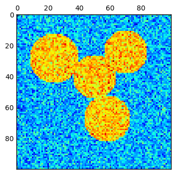
# 4 circles
img = circle1 + circle2 + circle3 + circle4
# We use a mask that limits to the foreground: the problem that we are
# interested in here is not separating the objects from the background,
# but separating them one from the other.
mask = img.astype(bool)
img = img.astype(float)
img += 1 + 0.2 * np.random.randn(*img.shape)
# Convert the image into a graph with the value of the gradient on the
# edges. 携带了梯度值,有什么用么?
graph = image.img_to_graph(img, mask=mask)
# Take a decreasing function of the gradient: we take it weakly
# dependent from the gradient the segmentation is close to a voronoi
graph.data = np.exp(-graph.data / graph.data.std())
# Force the solver to be arpack, since amg is numerically
# unstable on this example
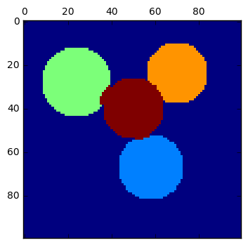
labels = spectral_clustering(graph, n_clusters=4, eigen_solver='arpack')
label_im = -np.ones(mask.shape)
label_im[mask] = labels
plt.matshow(img)
plt.matshow(label_im)
# #############################################################################
# 2 circles
img = circle1 + circle2
mask = img.astype(bool)
img = img.astype(float)
img += 1 + 0.2 * np.random.randn(*img.shape)
graph = image.img_to_graph(img, mask=mask)
graph.data = np.exp(-graph.data / graph.data.std())
labels = spectral_clustering(graph, n_clusters=2, eigen_solver='arpack')
label_im = -np.ones(mask.shape)
label_im[mask] = labels
plt.matshow(img)
plt.matshow(label_im)
plt.show()
Result:
算法理解:
# Convert the image into a graph with the value of the gradient on the
# edges. 携带了梯度值,有什么用么?
graph = image.img_to_graph(img, mask=mask)

# Take a decreasing function of the gradient: we take it weakly
# dependent from the gradient the segmentation is close to a voronoi
graph.data = np.exp(-graph.data / graph.data.std())

# Force the solver to be arpack, since amg is numerically
# unstable on this example
labels = spectral_clustering(graph, n_clusters=4, eigen_solver='arpack')
label_im = -np.ones(mask.shape)
label_im[mask] = labels
泰森多边形 voronoi

参考:Dimensionality Reduction: Why we take Eigenvectors of the Similarity Matrix?

 浙公网安备 33010602011771号