[Bayes] Maximum Likelihood estimates for text classification
Naïve Bayes Classifier.
We will use, specifically, the Bernoulli-Dirichlet model for text classification,
We will train the model using both the Maximum Likelihood estimates and Bayesian updating, and compare these in terms of predictive success, and in terms of what can go wrong.
We will be using the webkb dataset. - original data: the webkb dataset website.
[Scikit-learn] 1.9 Naive Bayes
[ML] Naive Bayes for Text Classification
[ML] Naive Bayes for email classification
In [31]:
# Make division default to floating-point, saving confusion
# i.e. 3/4 = 0.75 3//4 = 0
from __future__ import division

# Necessary libraries
import scipy as sp
import numpy as np
import matplotlib.pyplot as pl

# Put the graphs where we can see them
# 将matplotlib的图表直接嵌入到Notebook之中
%matplotlib inline

# Display a warning on important floating-point errors
np.seterr(divide='warn', invalid='warn');    # -->
Data 加载
In [32]:
data = np.load(
    'webkb.npz',
)

print(type(data))

# training data
xtrain = data['xtrain']
ytrain = data['ytrain']

# test data
xtest = data['xtest']
ytest = data['ytest']

# which class is which?
class_label_strings = data['class_label_strings']

# we don't need the original any more
del(data)
In [33]:
print("X training data dimensions = {!r}".format(xtrain.shape))    # -->
print("Y training data dimensions = {!r}".format(ytrain.shape))
print("X test data dimensions     = {!r}".format(xtest.shape))
print("Y test data dimensions     = {!r}".format(ytest.shape))
print("Number of y labels         = {!r}".format(len(class_label_strings)))
In [37]:
xtrain
Out[37]:
In [39]:
xtrain.shape[1]
Out[39]:
In [38]:
np.arange(xtrain.shape[0])
Out[38]:
In [75]:
# 行内求和
np.sum(xtrain, axis=0)
Out[75]:
In [74]:
# 列内求和
np.sum(xtrain, axis=1)
Out[74]:


array([ 12, 132, 102,  26, 107,  35,  34,  73,  69,  41,  41, 155,  58,
       239,  49, 129,  54, 126,  55, 242,  57,  83,  70, 108, 202,  51,
        79,  64, 134, 161, 107,  59, 204,  51,  63, 130,  47,  44,  45,
       161,  49,  67, 122,  58,  79,  45,  48,  55,  40,  65,  71,  95,
        23, 104,  87,  74, 261,  18,  85,  95,  25,  24,  64,  77,  49,
        46,  79,  46, 120,  78, 129,  97,  95,  30, 129, 177,  74,  56,
        70,  37, 175,  56, 210, 178, 161,  67,  70, 188,  51, 131,  59,
        26,  84,  75, 152,  35, 152, 100, 179,  86,  51, 249, 139,  80,
        51, 216,  41,  51,  56, 203, 196, 149,  39,  79,  49,  69, 101,
       133, 232,  78,  82, 196,  70, 157,  52, 113,  70,  66,  14, 111,
        88,  68, 183, 136,  57, 368,  48, 153,  44,  54,  95, 167,  79,
        96,  61, 106,  55,  96, 172, 171,  55, 105, 257,  41,  95,  65,
        61, 104,  43, 150, 210,  99,  66, 101, 151,  39,  46,  61, 160,
        69, 147,  20,  48,  70, 101,  76, 157,  66, 165,  80,  74,  26,
       148,  79,  55,  94,  47,  65, 103,  42,  51,  98,  51,  73,  36,
        90, 233,  57,  39,  71, 112,  55,  36,  81,  46, 132,  94, 141,
        98,  53,  84,  77,  87, 195, 200,  21,  69,  86,  85,  56,  51,
        68, 133, 109,  71,  70,  50,  88,  27, 107, 104,  75,  36,  61,
        90,  92,  32,  70,   4,  92,  79,  47,  73, 124,  46,  25, 106,
        78,  63,  97,  28, 106,  35,  61, 105,  48,  43, 276,  45,  40,
        69,  87, 120,  51,  40,  25, 116,  83,  51,  59, 162, 119, 168,
       161,  76,  87,  53,  63, 122, 138,  45,  54, 125, 115, 129,  83,
        70,  37, 209, 100,  68,  85,  87,  88,  23,  80, 129,  79,  85,
        67,  19,  90,  97, 167,  54, 149, 142,  85,  22,  78, 110, 129,
        87,  24,  82,  54,  91,  39,  55, 116, 142,  78,  62, 102,  44,
       231,  73,  95,  56, 121,  48, 116,  62,  81,  74,  50,  46,  77,
        61,  73,  68,  67,  67,  47,  61,  91,  95,  56,  51, 115, 125,
        91,  62,  48,  34, 177, 118,  71, 109,  56, 107, 208,  81, 419,
        88,  80, 262,  15,  87,  34,  42,  68,  40,  83, 128, 131,  82,
        67,  39, 138, 173, 101,  89,  21,  21,  65,  22,  32,  76, 101,
        60,  25,  39, 129,  32, 132, 141,  75,  22, 166,  95, 134, 241,
        87,  39, 132,  97,  77,  77,  68,  76, 100,  41,  80,  58, 134,
       102, 279,  29,  74, 114,  32,  16, 141, 100, 118,  70,  96,  32,
        70, 276,  93,  14,  70,  63,  55, 190,  45, 211,  66, 145,  37,
        88, 163,  79,  61,  46,  94, 112,  15,  94, 120,  69,  89,  58,
        71, 244,  24,  85,  88,  81,  54,  90, 152,  85,  68, 129,  56,
        84,  94,  82, 100,  71,  21, 199, 124,  66, 146,  31, 106,  48,
        49, 212,  93, 195,  46,  34,  15,  42,  88, 150,   1, 219,  62,
        49,  63,  47,  83, 100, 191,  72,  30,  72, 126,  72,  51,  36,
        99,  63, 146,  68, 117,  85, 114, 263,  26,  40, 137, 104, 100,
        71,  71,  29,  71,   1, 107,  56,  79, 104, 120, 162, 112,  61,
        90,  90,  63,  82, 101,  66,  73,  44, 160,  47,  66, 106,  81,
        59,  49,  99,  31,  58,  90,  61,  77,  34, 156,  22,  53,  80,
       237,  65,  35, 118,  87, 154,  71,  56,  51,  60, 184,  46,  80,
       105,  60, 160, 101,  95,  56, 345,  50, 103,  47,  76,  95,  96,
        68, 134, 103, 100,  51,  66,  27,  58,  52, 174, 111,  62, 304,
        67,  34, 107,  76, 181,  74,  75,  70,  26, 125,  54, 141, 165,
        44, 148, 106,  61,  26, 106,  24, 109, 164,  42, 125, 101,  51,
        94,  94, 130,  46,  75, 148, 105, 102,  45,  75, 192,  94, 157,
        24,  47, 136, 109, 153, 122,  93,  85,  77,  87,  24,  42, 114,
        32, 167, 121,  89,  44, 136, 110,  28, 174,  80,  66,  58,  93,
        88,  67,  84,  50, 341, 296,  24,  46,  38,  90,  48, 108, 204,
       201,  33,  88, 232, 226,  28, 104,  70,  44, 129, 286, 124,  73,
        43, 200,  39,  67,  39,  95, 106,  24,  77,  25,  71,  58, 187], dtype=uint64)
In [53]:
pl.bar( np.arange(xtrain.shape[1]), np.sum(xtrain, axis=0), width=1);

显示特定类别数据
In [78]:
# 提取 所有y样本中的第二项,也就是类别=2的样本;xtrain的第二维数据全要
x2 = xtrain[ytrain[:, 2]==1, :]
In [77]:
pl.bar( np.arange(x2.shape[1]), np.mean(x2, axis=0), width=1, alpha=0.5);

In [56]:
x3 = xtrain[ytrain[:, 3]==1, :]
pl.bar(np.arange(x3.shape[1]), np.mean(x3, axis=0), width=1, alpha=0.5);    # -->

# 其实就是只关心一部分数据(效果就是放大了),这里只关注前100个terms
In [57]:
pl.bar(np.arange(100), np.mean(x2[:, :100], axis=0), width=1, alpha=0.5);
pl.bar(np.arange(100), np.mean(x3[:, :100], axis=0), width=1, alpha=0.5);

Data Y 剖析
In [ ]:
def categorical_bar(val, **kwargs):
    """
    Convenient categorical bar plot, labelled with the class strings.
    This is handy if you want to plot something versus class.
    """
    n_cat = len(class_label_strings)
    cat_index = np.arange(n_cat)
    bar = pl.bar(cat_index, val, width=1, **kwargs);
    pl.xticks(cat_index, class_label_strings)
    return bar
In [8]:
categorical_bar(np.sum(ytrain, axis=0));

或者,直接返回数值形式
In [9]:
for label_string, n_in_class in zip(class_label_strings, np.sum(ytrain, axis=0)):
    print("{}: {}".format(label_string, n_in_class))
Maximum Likelihood Naïve Bayes Classifier

只是简单地求了平均值,过于naive的方法了啦。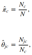
def fit_naive_bayes_ml(x, y):
    """
    Given an array of features `x` and an array of labels `y`,
    return ML estimates of class probabilities `pi` and
    class-conditional feature probabilities `theta`.
    """
    n_class = y.shape[1]
    n_feat  = x.shape[1]

    print(n_feat)
    print( len(x[0]) )

    pi_counts = np.sum(y, axis=0)
    print(pi_counts)

    #pi = pi_counts/np.sum(pi_counts)
    #print(pi)

    # 也可以通过 np.sum(y)直接求得matrix所有元素的总和
    pi = pi_counts/np.sum(y)
    print("pi: ", pi)

    print((n_feat, n_class))
    theta = np.zeros( (n_feat, n_class) )
    print("theta: ", theta)

    for cls in range(n_class):
        docs_in_class = (y[:, cls]==1)
        # 处理某一个特定类的train data,这里统计了该类下的单词在文档中的出现次数
        class_feat_count = x[docs_in_class, :].sum(axis=0)
        # Matrix求总和的两种方式:np.sum(...), x.sum()
        theta[:, cls] = class_feat_count/(docs_in_class.sum())
        # theta[:, cls] = class_feat_count/np.sum(docs_in_class)
    return pi, theta
pi_hat, theta_hat = fit_naive_bayes_ml(xtrain, ytrain)

print("pi_hat:    ", pi_hat)
print("theta_hat: ", theta_hat)
运行结果:
1703
1703
[ 165.   99.  345.   62.   31.]
('pi: ', array([ 0.23504274,  0.14102564,  0.49145299,  0.08831909,  0.04415954]))
(1703, 5)
('theta: ', array([[ 0.,  0.,  0.,  0.,  0.],
       [ 0.,  0.,  0.,  0.,  0.],
       [ 0.,  0.,  0.,  0.,  0.],
       ...,
       [ 0.,  0.,  0.,  0.,  0.],
       [ 0.,  0.,  0.,  0.,  0.],
       [ 0.,  0.,  0.,  0.,  0.]]))
('pi_hat:    ', array([ 0.23504274,  0.14102564,  0.49145299,  0.08831909,  0.04415954]))
('theta_hat: ', array([[ 0.01818182,  0.04040404,  0.00289855,  0.        ,  0.        ],
       [ 0.        ,  0.01010101,  0.0115942 ,  0.        ,  0.03225806],
       [ 0.        ,  0.03030303,  0.00869565,  0.01612903,  0.        ],
       ...,
       [ 0.01212121,  0.        ,  0.0115942 ,  0.01612903,  0.03225806],
       [ 0.39393939,  0.45454545,  0.53913043,  0.43548387,  0.41935484],
       [ 0.        ,  0.        ,  0.        ,  0.        ,  0.        ]]))
这里拿出一个x做预测实验:
categorical_bar( predict_class_prob(xtest[0,:], pi_hat, theta_hat), color='orange' );
from scipy.misc import logsumexp

def predict_class_prob(x, pi, theta):

    class_feat_l = np.zeros_like(theta)

    # calculations in log space to avoid underflow

    # 只提取该样本中包含单词对应的theta值
    # 因为,本样本没出现的单词,没必要关心在此
    print(len(theta[x==1, :]))

    class_feat_l[x==1, :] = np.log(theta[x==1, :])
    class_feat_l[x==0, :] = np.log(1 - theta[x==0, :])

    class_l = class_feat_l.sum(axis=0) + np.log(pi)

    # logsumexp 等价于 np.log(np.sum(np.exp(a)))
    return np.exp(class_l - logsumexp(class_l))  # --> 原理是什么
测试这套模型的正确率 (在测试集):
test_correct_ml = predictive_accuracy(xtest, ytest, predict_class, pi_hat, theta_hat)
def predictive_accuracy(xdata, ydata, predictor, *args):
    """
    Given an N-by-D array of features `xdata`,
    an N-by-C array of one-hot-encoded true classes `ydata`
    and a predictor function `predictor`,
    return the proportion of correct predictions.

    We accept an additional argument list `args`
    that will be passed to the predictor function.
    """
    correct = np.zeros(xdata.shape[0])
    for i, x in enumerate(xdata):
        prediction = predictor(x, *args)
        correct[i] = np.all(ydata[i, :] == prediction)
    return correct.mean()
def predict_class(x, pi, theta):
    probs = predict_class_prob(x, pi, theta)
    print(probs)

    prediction = np.zeros_like(probs)
    # 返回最大概率对应的位置,也就是idx
    prediction[np.argmax(probs)] = 1

    return prediction
以上实验 基本是在批判max likelihood的弊端,也就是无穷大和0带来的各种问题。

 浙公网安备 33010602011771号