
[Scikit-learn] 2.1 Clustering - Gaussian mixture models & EM
原理请观良心视频:机器学习课程 Expectation Maximisation

Expectation-maximization is a well-founded statistical algorithm to get around this problem by an iterative process.
- First one assumes random components (randomly centered on data points, learned from k-means, or even just normally distributed around the origin) and computes for each point a probability of being generated by each component of the model.
- Then, one tweaks the parameters to maximize the likelihood of the data given those assignments. Repeating this process is guaranteed to always converge to a local optimum.
实战:
X_train
Out[79]:
array([[ 4.3,  3. ,  1.1,  0.1],
       [ 5.8,  4. ,  1.2,  0.2],
       [ 5.7,  4.4,  1.5,  0.4],
       ...,
       [ 6.5,  3. ,  5.2,  2. ],
       [ 6.2,  3.4,  5.4,  2.3],
       [ 5.9,  3. ,  5.1,  1.8]])

X_train.size
Out[80]: 444

classifier.means_
Out[81]:
array([[ 5.04594595,  3.45135126,  1.46486501,  0.25675684],    # 1st 4d Gaussian
       [ 5.92023012,  2.75827264,  4.42168189,  1.43882194],    # 2nd 4d Gaussian
       [ 6.8519452 ,  3.09214071,  5.71373857,  2.0934678 ]])   # 3rd 4d Gaussian

classifier.covars_
Out[82]:
array([[ 0.08532076,  0.08532076,  0.08532076,  0.08532076],
       [ 0.14443088,  0.14443088,  0.14443088,  0.14443088],
       [ 0.1758563 ,  0.1758563 ,  0.1758563 ,  0.1758563 ]])
本有四个变量,如何画在平面图上的呢?以上只取了前两维数据做图。
"""
==================
GMM classification
==================
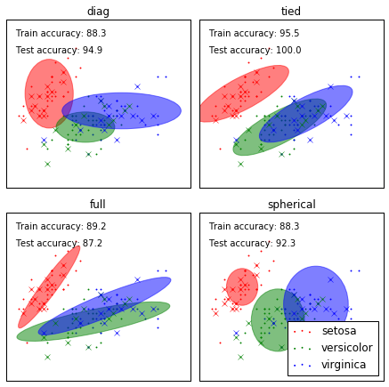
Demonstration of Gaussian mixture models for classification.
See :ref:`gmm` for more information on the estimator.
Plots predicted labels on both training and held out test data using a
variety of GMM classifiers on the iris dataset.
Compares GMMs with spherical, diagonal, full, and tied covariance
matrices in increasing order of performance. Although one would
expect full covariance to perform best in general, it is prone to
overfitting on small datasets and does not generalize well to held out
test data.
On the plots, train data is shown as dots, while test data is shown as
crosses. The iris dataset is four-dimensional. Only the first two
dimensions are shown here, and thus some points are separated in other
dimensions.
"""
print(__doc__)
# Author: Ron Weiss <ronweiss@gmail.com>, Gael Varoquaux
# License: BSD 3 clause
# $Id$
import matplotlib.pyplot as plt
import matplotlib as mpl
import numpy as np
from sklearn import datasets
from sklearn.cross_validation import StratifiedKFold
from sklearn.externals.six.moves import xrange
from sklearn.mixture import GMM
def make_ellipses(gmm, ax):
for n, color in enumerate('rgb'):
v, w = np.linalg.eigh(gmm._get_covars()[n][:2, :2])
u = w[0] / np.linalg.norm(w[0])
angle = np.arctan2(u[1], u[0])
angle = 180 * angle / np.pi # convert to degrees
v *= 9
ell = mpl.patches.Ellipse(gmm.means_[n, :2], v[0], v[1], 180 + angle, color=color)
ell.set_clip_box(ax.bbox)
ell.set_alpha(0.5)
ax.add_artist(ell)
iris = datasets.load_iris()
#数据预处理
# Break up the dataset into non-overlapping training (75%) and testing
# (25%) sets.
# 分层交叉验证,使得交叉验证抽到的样本符合原始样本的比例。
skf = StratifiedKFold(iris.target, n_folds=4)
# Only take the first fold.
train_index, test_index = next(iter(skf))
# next(iter())逐个遍历skf的elem, len(skf) = 4
# 随机获取了四组中的一组数据
X_train = iris.data [train_index]
y_train = iris.target[train_index]
X_test = iris.data [test_index]
y_test = iris.target[test_index]
#GMM初始化
n_classes = len(np.unique(y_train))
# y_train就三种值,代表有仨个Gaussian
# Try GMMs using different types of covariances.
# 四种不同的type做GMM,然后存放在dict中
classifiers = dict((covar_type,
GMM(n_components=n_classes, covariance_type=covar_type, init_params='wc', n_iter=20)
)
for covar_type in ['spherical', 'diag', 'tied', 'full']
)
# NB:covar_type的表现往往体现在高斯分布图像的旋转
n_classifiers = len(classifiers)
plt.figure(figsize=(3 * n_classifiers / 2, 6))
plt.subplots_adjust(bottom=.01, top=0.95, hspace=.15, wspace=.05,
left=.01, right=.99)
for index, (name, classifier) in enumerate(classifiers.items()):
"""
dict_items([('diag', GMM(covariance_type='diag', init_params='wc', min_covar=0.001, n_components=5, n_init=1, n_iter=20, params='wmc', random_state=None, tol=0.001, verbose=0)),
('tied', GMM(covariance_type='tied', init_params='wc', min_covar=0.001, n_components=5, n_init=1, n_iter=20, params='wmc', random_state=None, tol=0.001, verbose=0)),
('full', GMM(covariance_type='full', init_params='wc', min_covar=0.001, n_components=5, n_init=1, n_iter=20, params='wmc', random_state=None, tol=0.001, verbose=0)),
('spherical', GMM(covariance_type='spherical', init_params='wc', min_covar=0.001, n_components=5, n_init=1, n_iter=20, params='wmc', random_state=None, tol=0.001, verbose=0))])
"""
# 数据训练
    # Since we have class labels for the training data, we can
    # initialize the GMM parameters in a supervised manner.
    classifier.means_ = np.array([X_train[y_train == i].mean(axis=0) for i in xrange(n_classes)])
    # axis=0 沿着Matrix的‘行’求统计量,NB:每个向量的第一元素求mean,第二个元素求mean ...

    # Train the other parameters using the EM algorithm.
    classifier.fit(X_train)

# 数据表现
    h = plt.subplot(2, n_classifiers / 2, index + 1)
    make_ellipses(classifier, h)

for n, color in enumerate('rgb'):
        data = iris.data[iris.target == n]
       plt.scatter(data[:, 0], data[:, 1], 0.8, color=color,
                    label=iris.target_names[n])
    # Plot the test data with crosses
    for n, color in enumerate('rgb'):
        data = X_test[y_test == n]
        plt.plot(data[:, 0], data[:, 1], 'x', color=color)

    y_train_pred = classifier.predict(X_train)
    train_accuracy = np.mean(y_train_pred.ravel() == y_train.ravel()) * 100
    plt.text(0.05, 0.9, 'Train accuracy: %.1f' % train_accuracy,
             transform=h.transAxes)
    test_accuracy = np.mean(y_test_pred.ravel() == y_test.ravel()) * 100
    plt.text(0.05, 0.8, 'Test accuracy: %.1f' % test_accuracy,
             transform=h.transAxes)

    plt.xticks(())
    plt.yticks(())
    plt.title(name)

plt.legend(loc='lower right', prop=dict(size=12))

plt.show()
New api: mixture.GMM
"""
=============================================
Density Estimation for a mixture of Gaussians
=============================================

Plot the density estimation of a mixture of two Gaussians. Data is
generated from two Gaussians with different centers and covariance
matrices.
"""

import numpy as np
import matplotlib.pyplot as plt
from matplotlib.colors import LogNorm
from sklearn import mixture

n_samples = 300

# generate random sample, two components
np.random.seed(0)

# generate spherical data centered on (20, 20)
shifted_gaussian = np.random.randn(n_samples, 2) + np.array([20, 20])

# generate zero centered stretched Gaussian data
C = np.array([[0., -0.7], [3.5, .7]])
stretched_gaussian = np.dot(np.random.randn(n_samples, 2), C)

# concatenate the two datasets into the final training set
X_train = np.vstack([shifted_gaussian, stretched_gaussian])

# fit a Gaussian Mixture Model with two components
clf = mixture.GMM(n_components=2, covariance_type='full')
clf.fit(X_train)

# display predicted scores by the model as a contour plot
x = np.linspace(-20.0, 30.0)
y = np.linspace(-20.0, 40.0)
X, Y = np.meshgrid(x, y)
XX = np.array([X.ravel(), Y.ravel()]).T
Z = -clf.score_samples(XX)[0]
Z = Z.reshape(X.shape)

CS = plt.contour(X, Y, Z, norm=LogNorm(vmin=1.0, vmax=1000.0),
                 levels=np.logspace(0, 3, 10))
CB = plt.colorbar(CS, shrink=0.8, extend='both')
plt.scatter(X_train[:, 0], X_train[:, 1], .8)

plt.title('Negative log-likelihood predicted by a GMM')
plt.axis('tight')
plt.show()
如何判定模型中有几个Gaussian,Selecting the number of components in a classical GMM
The BIC criterion can be used to select the number of components in a GMM in an efficient way. In theory, it recovers the true number of components only in the asymptotic regime (i.e. if much data is available).
Note that using a DPGMM avoids the specification of the number of components for a Gaussian mixture model.
(NOTE:DPGMM会放在Dirichlet Process章节中学习)
哪个模型更加的好呢?目前常用有如下方法:
AIC = -2 ln(L) + 2k Akaike information criterion
BIC = -2 ln(L) + ln(n)*k Bayesian information criterion
HQ = -2 ln(L) + ln(ln(n))*k Hannan-quinn criterion
其中L是在该模型下的最大似然,n是数据数量,k是模型的变量个数。
注意这些规则只是刻画了用某个模型之后相对“真实模型”的信息损失【因为不知道真正的模型是什么样子,所以训练得到的所有模型都只是真实模型的一个近似模型】,所以用这些规则不能说明某个模型的精确度,即三个模型A, B, C,在通过这些规则计算后,我们知道B模型是三个模型中最好的,但是不能保证B这个模型就能够很好地刻画数据,因为很有可能这三个模型都是非常糟糕的,B只是烂苹果中的相对好的苹果而已。
这些规则理论上是比较漂亮的,但是实际在模型选择中应用起来还是有些困难的,例如上面我们说了5个变量就有32个变量组合,如果是10个变量呢?2的10次方,我们不可能对所有这些模型进行一一验证AIC, BIC,HQ规则来选择模型,工作量太大。
"""
=================================
Gaussian Mixture Model Selection
=================================

This example shows that model selection can be performed with
Gaussian Mixture Models using information-theoretic criteria (BIC).
Model selection concerns both the covariance type
and the number of components in the model.
In that case, AIC also provides the right result (not shown to save time),
but BIC is better suited if the problem is to identify the right model.
Unlike Bayesian procedures, such inferences are prior-free.

In that case, the model with 2 components and full covariance
(which corresponds to the true generative model) is selected.
"""
print(__doc__)

import itertools

import numpy as np
from scipy import linalg
import matplotlib.pyplot as plt
import matplotlib as mpl

from sklearn import mixture

# Number of samples per component
n_samples = 500

# Generate random sample, two components
np.random.seed(0)
C = np.array([[0., -0.1], [1.7, .4]])
X = np.r_[np.dot(np.random.randn(n_samples, 2), C),
          .7 * np.random.randn(n_samples, 2) + np.array([-6, 3])]

lowest_bic = np.infty
bic = []
n_components_range = range(1, 7)
cv_types = ['spherical', 'tied', 'diag', 'full']
for cv_type in cv_types:
    for n_components in n_components_range:
        # Fit a mixture of Gaussians with EM
        gmm = mixture.GMM(n_components=n_components, covariance_type=cv_type)
        gmm.fit(X)
        bic.append(gmm.bic(X))
        if bic[-1] < lowest_bic:
            lowest_bic = bic[-1]
            best_gmm   = gmm

# 这里不需要 test set

bic = np.array(bic)
color_iter = itertools.cycle(['k', 'r', 'g', 'b', 'c', 'm', 'y'])
clf = best_gmm
bars = []

# Plot the BIC scores
spl = plt.subplot(2, 1, 1)
for i, (cv_type, color) in enumerate(zip(cv_types, color_iter)):
    xpos = np.array(n_components_range) + .2 * (i - 2)
    bars.append(plt.bar(xpos, bic[i * len(n_components_range):
                                  (i + 1) * len(n_components_range)],
                        width=.2, color=color))
plt.xticks(n_components_range)
plt.ylim([bic.min() * 1.01 - .01 * bic.max(), bic.max()])
plt.title('BIC score per model')
xpos = np.mod(bic.argmin(), len(n_components_range)) + .65 +\
    .2 * np.floor(bic.argmin() / len(n_components_range))
plt.text(xpos, bic.min() * 0.97 + .03 * bic.max(), '*', fontsize=14)
spl.set_xlabel('Number of components')
spl.legend([b[0] for b in bars], cv_types)

# Plot the winner
splot = plt.subplot(2, 1, 2)
Y_ = clf.predict(X)
for i, (mean, covar, color) in enumerate(zip(clf.means_, clf.covars_,
                                             color_iter)):
    v, w = linalg.eigh(covar)
    if not np.any(Y_ == i):
        continue
    plt.scatter(X[Y_ == i, 0], X[Y_ == i, 1], .8, color=color)

    # Plot an ellipse to show the Gaussian component
    angle = np.arctan2(w[0][1], w[0][0])
    angle = 180 * angle / np.pi  # convert to degrees
    v *= 4
    ell = mpl.patches.Ellipse(mean, v[0], v[1], 180 + angle, color=color)
    ell.set_clip_box(splot.bbox)
    ell.set_alpha(.5)
    splot.add_artist(ell)

plt.xlim(-10, 10)
plt.ylim(-3, 6)
plt.xticks(())
plt.yticks(())
plt.title('Selected GMM: full model, 2 components')
plt.subplots_adjust(hspace=.35, bottom=.02)
plt.show()

 浙公网安备 33010602011771号