[ML] Naive Bayes for Text Classification
TF-IDF Algorithm
From http://www.ruanyifeng.com/blog/2013/03/tf-idf.html
原理概述
"词频"(TF)
考虑“词”,分母也可以是“文章总词数”。

"逆文档频率"(Inverse Document Frequency,缩写为IDF)
如果某个词比较少见,但是它在这篇文章中多次出现,那么它很可能就反映了这篇文章的特性,正是我们所需要的关键词。
"逆文档频率"(Inverse Document Frequency,缩写为IDF),它的大小与一个词的常见程度成反比。
考虑“文档”。

计算TF-IDF
知道了"词频"(TF)和"逆文档频率"(IDF)以后,将这两个值相乘,就得到了一个词的TF-IDF值。某个词对文章的重要性越高,它的TF-IDF值就越大。

Pros and cons
优点: 是简单快速,结果比较符合实际情况。
缺点: 是,单纯以"词频"衡量一个词的重要性,不够全面,
-
- 重要的词可能出现次数并不多。
- 这种算法无法体现词的位置信息,出现位置靠前的词与出现位置靠后的词,都被视为重要性相同,这是不正确的。可以对全文的第一段和每一段的第一句话,给予较大的权重。
余弦相似性
From http://www.ruanyifeng.com/blog/2013/03/cosine_similarity.html
我们的目的
先从简单的句子着手。
句子A:我喜欢看电视,不喜欢看电影。
句子B:我不喜欢看电视,也不喜欢看电影。
基本步骤
词频向量
基本思路是:如果这两句话的用词越相似,它们的内容就应该越相似。因此,可以从词频入手,计算它们的相似程度。
Step 1,分词。
句子A:我/喜欢/看/电视,不/喜欢/看/电影。
句子B:我/不/喜欢/看/电视,也/不/喜欢/看/电影。
Step 2,列出所有的词。
我,喜欢,看,电视,电影,不,也。
Step 3,计算词频。
句子A:我 1,喜欢 2,看 2,电视 1,电影 1,不 1,也 0。
句子B:我 1,喜欢 2,看 2,电视 1,电影 1,不 2,也 1。
Step 4,写出词频向量。
句子A:[1, 2, 2, 1, 1, 1, 0]
句子B:[1, 2, 2, 1, 1, 2, 1]
到这里,问题就变成了如何计算这两个向量的相似程度。
两条线段之间形成一个夹角,我们可以通过夹角的大小,来判断向量的相似程度。夹角越小,就代表越相似。
- 如果夹角为0度,意味着方向相同、线段重合;
- 如果夹角为90度,意味着形成直角,方向完全不相似;
- 如果夹角为180度,意味着方向正好相反。// impossible
向量夹角计算
以二维空间为例,上图的a和b是两个向量,我们要计算它们的夹角θ。参考:余弦定理 
余弦值越接近1,就表明夹角越接近0度,也就是两个向量越相似,这就叫"余弦相似性"。所以,上面的句子A和句子B是很相似的,事实上它们的夹角大约为20.3度。
由此,我们就得到了"找出相似文章"的一种算法:
(1)使用TF-IDF算法,找出两篇文章的关键词;
(2)每篇文章各取出若干个关键词(比如20个),合并成一个集合,计算每篇文章对于这个集合中的词的词频(为了避免文章长度的差异,可以使用相对词频);
(3)生成两篇文章各自的词频向量;
(4)计算两个向量的余弦相似度,值越大就表示越相似。
"余弦相似度"是一种非常有用的算法,只要是计算两个向量的相似程度,都可以采用它。
Step by Step 改进 "朴素贝叶斯"
From http://blog.csdn.net/ehomeshasha/article/details/35988111
朴素贝叶斯表达式
多项式朴素贝叶斯 (multinomial Naive Bayes)
对于其中的某个类别c来说
多项式系数表达为:


某个单词在类别c中出现的可能性,所以其加和必然为1,公式为
MAP假设以及将值取log:
在上面的公式中,


/* 具体详见原链接 */
互补朴素贝叶斯 (Complement naive Bayes)
From http://stats.stackexchange.com/questions/126009/complement-naive-bayes
举个例子:文档内容,文档类别
Let's say we have three documents with the following words:
// training
Doc 1: "Food" occurs 2 times, "Meat" occurs 1 time, "Brain" occurs 1 time --> 4
Class of Doc 1: "Health"

Doc 2: "Food" occurs 1 time, "Meat" occurs 1 time, "Kitchen" occurs 9 times, "Job" occurs 5 times. --> 16
Class of Doc 2: "Butcher"

Doc 3: "Food" occurs 2 times, "Meat" occurs 1 time, "Job" occurs 1 time. --> 4
Class of Doc 3: "Health"
一个word属于俩类别的先验概率
Total word count in class 'Health' - (2+1+1)+(2+1+1) = 8
Total word count in class 'Butcher' - (1+1+9+5) = 16
So we have two possible y classes: (y=Health) and (y=Butcher) , with prior probabilities thus:
p(y=Health) = 2/3 (2 out of 3 docs are about Health)
p(y=Butcher) = 1/3
互补概率
Now, for Complement Normal Naive Bayes, instead of calculating the likelihood of a word occuring in a class,
we calculate the likelihood that it occurs in other classes. So, we would proceed to calculate the word-class dependencies thus:
Complement Probability of word 'Food' with class 'Health':
p( w=Food | ŷ=Health ) = 1/16
See? 'Food' occurs 1 time in total for all classes NOT health, and the number of words in class NOT health is 16.
Complement Probability of word 'Food' with class 'Butcher':
p( w=Food | ŷ=Butcher ) = (2+2)/8 = 0.5
For others,
p( w=Kitchen | ŷ =Health ) = 9/16
p( w=Kitchen | ŷ =Butcher) = 0/8 = 0
p( w=Meat | ŷ =Health    ) = 1/16
p( w=Meat | ŷ =Butcher   ) = 2/8
...and so forth
预测新文档
New doc:
"Food" - 1, "Job" - 1, "Meat" - 1
Then, say we had a new document containing the following:
(1)

(2)

We would predict the class of this new doc by doing the following:
which gives us

Let's work it out - this will give us:


...and likewise for the other classes.
So, the one with the lower probability (minimum value) is said to be the class it belongs to - in this case,
our new doc will be classified as belonging to Health.
We DON'T use the one with the maximum probability because for the Complement Naive Bayes Algorithm, we take it - a higher value - to mean that it is highly likely that a document with these words does NOT belong to that class.
Obviously, this example is, again, highly contrived, and we should even talk about Laplacian smoothing. But hope this helps you have a working idea on which you can build!
贝叶斯"隐变量"模型
模型概览
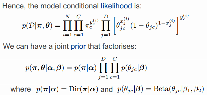
本文考虑了先验分布
Ref: [Bayesian] “我是bayesian我怕谁”系列 - Naive Bayes with Prior
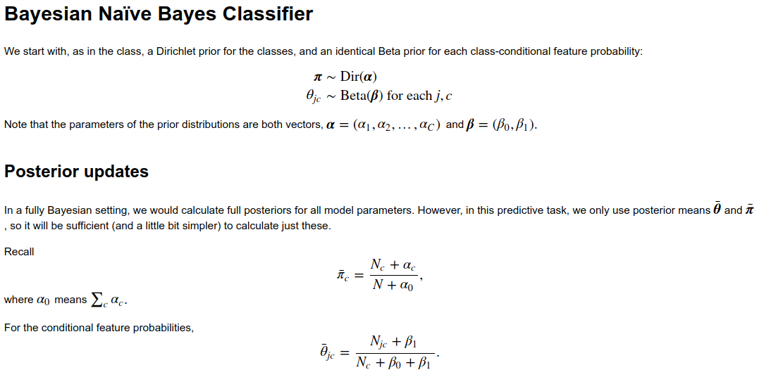
多项式分布的先验:Dir分布;二项分布的先验:Bate分布。

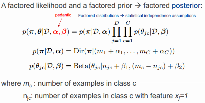
然后,得到俩参数的后验:

参数后验分布的期望就是预测值:

模型估参
def naive_bayes_posterior_mean(x, y, alpha=1, beta=1):

    n_class = y.shape[1]
    n_feat  = x.shape[1]

    # alpha的设置,不需要搞一个长向量,因为初始是平均的;
    # but for beta, we must be explicit
    beta = np.ones(2) * beta

    # 直接套入pi的后验结论
    pi_counts = np.sum(y, axis=0) + alpha
    pi        = pi_counts/np.sum(pi_counts)

    # 直接套入theta的后验结论
    theta     = np.zeros((n_feat, n_class))

    for cls in range(n_class):
        docs_in_class = (y[:, cls]==1)
        class_feat_count = x[docs_in_class, :].sum(axis=0)
        theta[:, cls] = (class_feat_count + beta[1])/(docs_in_class.sum() + beta.sum())

    return pi, theta
pi_bar, theta_bar = naive_bayes_posterior_mean(xtrain, ytrain, alpha=1, beta=1)
print(pi_bar)       # Cat(y|pi)
print(theta_bar)    # Ber(xj|thetajc)
Result:
[ 0.23479491  0.14144272  0.4893918   0.08910891  0.04526167]

[[ 0.0239521   0.04950495  0.00576369  0.015625    0.03030303]  # 生成式概率:第c类的topic包含这个单词的概率是多大
 [ 0.00598802  0.01980198  0.01440922  0.015625    0.06060606]
 [ 0.00598802  0.03960396  0.01152738  0.03125     0.03030303]
 ...,
 [ 0.01796407  0.00990099  0.01440922  0.03125     0.06060606]
 [ 0.39520958  0.45544554  0.5389049   0.4375      0.42424242]  # stop word可能会是这样的概率状况,在每个topic中以较高的概率存在其身影
 [ 0.00598802  0.00990099  0.00288184  0.015625    0.03030303]]
模型预测
from scipy.misc import logsumexp

def predict_class_prob(x, pi, theta):


    # 哪个类概率大,就预测是哪个类
    class_feat_l = np.zeros_like(theta)

    # calculations in log space to avoid underflow
    class_feat_l[x==1, :] = np.log(theta[x==1, :])
    class_feat_l[x==0, :] = np.log(1 - theta[x==0, :])

    class_l = class_feat_l.sum(axis=0) + np.log(pi)
    # class_1: predict的log后的结果# logsumexp 等价于 np.log(np.sum(np.exp(a)))
    return np.exp(class_l - logsumexp(class_l)) #--> 返回的就是归一化后的概率比值


# 这个返回决策结果
def predict_class(x, pi, theta):
    """
    Given a feature vector `x`, class probabilities `pi`
    and class-conditional feature probabilities `theta`,
    return a one-hot encoded MAP class-membership prediction.
    """
    probs = predict_class_prob(x, pi, theta)

    prediction = np.zeros_like(probs)
    prediction[np.argmax(probs)] = 1
    return prediction
def predictive_accuracy(xdata, ydata, predictor, *args):
    """
    Given an N-by-D array of features `xdata`,
    an N-by-C array of one-hot-encoded true classes `ydata`
    and a predictor function `predictor`,
    return the proportion of correct predictions.

    We accept an additional argument list `args`
    that will be passed to the predictor function.
    """
    correct = np.zeros(xdata.shape[0])
    for i, x in enumerate(xdata):
        prediction = predictor(x, *args)
        correct[i] = np.all(ydata[i, :] == prediction)  # 判断运算符,拿出ydata的对应的行,与prediction的五个元素比较后都对才叫对
    return correct.mean()
# 预测第48条样本
categorical_bar(predict_class_prob( xtest[48,:], pi_bar, theta_bar), alpha=0.5, color='orange' );
categorical_bar(ytest[48,:], alpha=0.5, color='blue');
# 预测所有样本,查看预测总体效果
train_correct_bayes = predictive_accuracy(xtrain, ytrain, lambda x: predict_class(x, pi_bar, theta_bar))
print("Full Bayes In-sample proportion correct: {:.3}".format(train_correct_bayes))

test_correct_bayes = predictive_accuracy(xtest, ytest, lambda x: predict_class(x, pi_bar, theta_bar))
print("Full Bayes Out-of-sample proportion correct: {:.3}".format(test_correct_bayes))
先验初始值对结果的影响
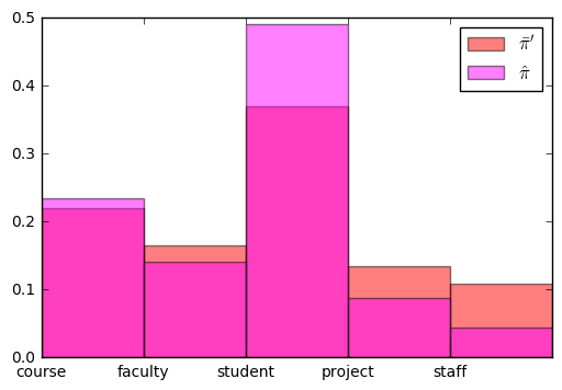
比如扩大:α=(100,100,…,100).
pi_bar_10, theta_bar_10 = naive_bayes_posterior_mean(xtrain, ytrain, alpha=100, beta=1)

categorical_bar(pi_bar_10, color='red', alpha=0.5, label=r"$\bar{\pi}'$");
categorical_bar(pi_hat, color='magenta', alpha=0.5, label=r'$\hat{\pi}$');
pl.legend();
Result:看上去更加均匀,成为了pi的后验期望的主导。

20 Newsgroups
Dataset: http://qwone.com/~jason/20Newsgroups/
1. Introduction
This is only a test report for naive bayes algorithm on email classification, which will help you to further understand Naive Bayes.
The goal is to implement a version of the Naive Bayes classifier and apply it to the text documents in the 20 newgroups data set, which is a collection of approximately 20,000 newsgroup documents, partitioned (nearly) evenly across 20 different newsgroups.
2. Method
Here, three Impact Factors are considered to improve the accuracy of classification.
(1) Adopt the same approach as described in Chapter 6 of Mitchell's book as following.

(2) Filter out the high frequency words which are useless for recognition, such as 'the', 'is', etc. The word found in more groups, its weight value will be smaller. Thus the method of TF-IDF (term frequency–inverse document frequency) will be considered.
(3) The probability of a word occurring is dependent of its position within the text, so next, the weight value of position for each word is considered.
In order to keep implementation simple, it simply assumes that:
(a) the importance of words in an email is descending,
(b) but key words will be repeated at the end of email.
Gaussian distributions is used to describe the importance. The horizontal axis shows word position in main body of email. The vertical axis represents the importance. Thus, two Gaussian distributions will represent these two assumptions respectively. The importance of one word will be the result of accumulation between two values from these two assumptions.
Two group of proper parameters for two Gaussian distributions will be determined based on lots of test.

Otherwise, we use log rule as below to transform division to subtraction for avoiding the problem of arithmetic underflow caused by the tiny probability.
log(a/b) = log(a) - log(b)
Next, according to the log rule, three Impact Factors can determine the word probability in each group in the form as following:
Word Probability = log(“impact factor 1”) + log(“impact factor 2”) + log(“impact factor 3”)
Considering that the importance of these Impact Factors are different, thus we need to find proper weight value for each of them to get a maximum of accuracy of classification. So, the form will be as following:
Word Probability = weight1×log(“impact factor 1”) + weight2×log(“impact factor 2”) + weight3×log(“impact factor 3”)
3. Results
After implement of 1st Impact Factor, the accuracy of classification is about 73.81%.
After implement of 2nd Impact Factor, surprisingly there is no improvement on accuracy.
In 3rd Impact Factor, there are three groups of uncertain values that we should test to find the proper values.
Finally, we have got the proper parameters and weight values to achieve the accuracy of 81.12%.
4. Discussion
TF-IDF doesn't work here. It possibly shows that the high frequency words are evenly distributed in each group.
Here, it is only a simple assumption on the importance of word position and this Impact Factor has good performance on accuracy improvement. I think, there are still better assumptions which have better performance, for example: “the first paragraph and the first sentence in each paragraph are important.” However, this assumption needs much more time to implement due to the non-unified format of main body in email.
5. Conclusions
The Naive Bayes classifier has a good performance on email classification and the analysis on word position will further improve the accuracy. The probability of guessing the group is 5% (1/20) and the algorithm above achieves 81.12%.
6. References
Mitchell, T. "Machine Learning". McGraw Hill, 1997.


 浙公网安备 33010602011771号