[Feature] Feature selection - Embedded topic
基于惩罚项的特征选择法
一、直接对特征筛选
Ref: 1.13.4. 使用SelectFromModel选择特征(Feature selection using SelectFromModel)
通过 L1 降维特征
L1惩罚项降维的原理在于保留多个对目标值具有同等相关性的特征中的一个,所以没选到的特征不代表不重要。故,可结合L2惩罚项来优化。
(1) [Scikit-learn] 1.1 Generalized Linear Models - from Linear Regression to L1&L2【as part 1】
(2) [Scikit-learn] 1.1 Generalized Linear Models - Lasso Regression【as part 2,重点解析了Lasso,作为part 1的补充】
示例代码如下,但问题来了,如何图像化参数的重要性。
from sklearn.svm import LinearSVC

X.shape
# (150, 4)

lsvc = LinearSVC(C=0.01, penalty="l1", dual=False).fit(X, y)
model = SelectFromModel(lsvc, prefit=True)

# 原数据 --> 转变为 --> 降维后的数据
X_new = model.transform(X)
X_new.shape
# (150, 3)
L1 参数筛选
直接得到理想的模型,查看最后参数的二维分布:Feature selection using SelectFromModel and LassoCV
# Author: Manoj Kumar <mks542@nyu.edu>
# License: BSD 3 clause

print(__doc__)

import matplotlib.pyplot as plt
import numpy as np

from sklearn.datasets import load_boston
from sklearn.feature_selection import SelectFromModel
from sklearn.linear_model import LassoCV

# Load the boston dataset.
boston = load_boston()
X, y = boston['data'], boston['target']

# We use the base estimator LassoCV since the L1 norm promotes sparsity of features.
clf = LassoCV()

# Set a minimum threshold of 0.25
sfm = SelectFromModel(clf, threshold=0.25)
sfm.fit(X, y)
n_features = sfm.transform(X).shape[1]

# Reset the threshold till the number of features equals two.
# Note that the attribute can be set directly instead of repeatedly
# fitting the metatransformer.
while n_features > 2:
    sfm.threshold += 0.1
    X_transform = sfm.transform(X)
    n_features = X_transform.shape[1]

# Plot the selected two features from X.
plt.title(
    "Features selected from Boston using SelectFromModel with "
    "threshold %0.3f." % sfm.threshold)
feature1 = X_transform[:, 0]
feature2 = X_transform[:, 1]
plt.plot(feature1, feature2, 'r.')
plt.xlabel("Feature number 1")
plt.ylabel("Feature number 2")
plt.ylim([np.min(feature2), np.max(feature2)])
plt.show()
二、轨迹图
Sparse recovery: feature selection for sparse linear models
学习可视化 L1 过程,代码分析。
Ref: Lasso权重可视化
注意,该标题的代码过期了:Deprecate randomized_l1 module #8995
轨迹图
Ref: LARS算法的几何意义
Ref: 1.1. Generalized Linear Models【更多轨迹图】
从右往左看,重要的参数在最后趋于0。
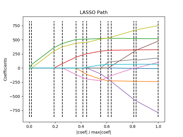
print(__doc__)

# Author: Fabian Pedregosa <fabian.pedregosa@inria.fr>
#         Alexandre Gramfort <alexandre.gramfort@inria.fr>
# License: BSD 3 clause

import numpy as np
import matplotlib.pyplot as plt

from sklearn import linear_model
from sklearn import datasets

diabetes = datasets.load_diabetes()
X = diabetes.data
y = diabetes.target

print("Computing regularization path using the LARS ...")
_, _, coefs = linear_model.lars_path(X, y, method='lasso', verbose=True)


# 注释一:累加,然后变为“比例”
xx = np.sum(np.abs(coefs.T), axis=1)
xx /= xx[-1]


plt.plot(xx, coefs.T)
ymin, ymax = plt.ylim()
plt.vlines(xx, ymin, ymax, linestyle='dashed')
plt.xlabel('|coef| / max|coef|')
plt.ylabel('Coefficients')
plt.title('LASSO Path')
plt.axis('tight')
plt.show()
“注释一” 的结果显示:
Computing regularization path using the LARS ...

[   0.           60.11926965  663.66995526  888.91024335 1250.6953637
 1440.79804251 1537.06598321 1914.57052862 2115.73774356 2195.55885543
 2802.37509283 2863.01080401 3460.00495515]

[0.         0.01737549 0.19181185 0.25691011 0.36147213 0.41641502
 0.44423809 0.55334329 0.61148402 0.63455367 0.80993384 0.82745858
 1.        ]
三、L2 协助 L1 优化
L1惩罚项降维的原理在于保留多个对目标值具有同等相关性的特征中的一个,所以没选到的特征不代表不重要。故,可结合L2惩罚项来优化。
具体操作为:若一个特征在L1中的权值为1,选择在L2中权值差别不大且在L1中权值为0的特征构成同类集合,将这一集合中的特征平分L1中的权值,故需要构建一个新的逻辑回归模型:
-
- __init__中,默认L1, 但内部又“配置了一个L2"的额外的模型。
- fit()进行了重写:先用L1训练一次,再用L2训练一次。
from sklearn.linear_model import LogisticRegression

class LR(LogisticRegression):

    def __init__(self, threshold=0.01, dual=False, tol=1e-4, C=1.0,
                 fit_intercept=True, intercept_scaling=1, class_weight=None,
                 random_state=None, solver='liblinear', max_iter=100,
                 multi_class='ovr', verbose=0, warm_start=False, n_jobs=1):

        #权值相近的阈值
        self.threshold = threshold

        #初始化模型
        LogisticRegression.__init__(self, penalty='l1', dual=dual, tol=tol, C=C,
                 fit_intercept=fit_intercept, intercept_scaling=intercept_scaling, class_weight=class_weight,
                 random_state=random_state, solver=solver, max_iter=max_iter,
                 multi_class=multi_class, verbose=verbose, warm_start=warm_start, n_jobs=n_jobs)

        #使用同样的参数创建L2逻辑回归
        self.l2 = LogisticRegression(penalty='l2', dual=dual, tol=tol, C=C, fit_intercept=fit_intercept, intercept_scaling=intercept_scaling, class_weight = class_weight, random_state=random_state, solver=solver, max_iter=max_iter, multi_class=multi_class, verbose=verbose, warm_start=warm_start, n_jobs=n_jobs)


    def fit(self, X, y, sample_weight=None):

        #训练L1逻辑回归
        super(LR, self).fit(X, y, sample_weight=sample_weight)
        self.coef_old_ = self.coef_.copy()

        #训练L2逻辑回归
        self.l2.fit(X, y, sample_weight=sample_weight)

        cntOfRow, cntOfCol = self.coef_.shape

        # 权值系数矩阵的行数对应目标值的种类数目
        for i in range(cntOfRow):
            for j in range(cntOfCol):

                coef = self.coef_[i][j]
                #L1逻辑回归的权值系数不为0
                if coef != 0:
                    idx = [j]
                    #对应在L2逻辑回归中的权值系数
                    coef1 = self.l2.coef_[i][j]
                    for k in range(cntOfCol):
                        coef2 = self.l2.coef_[i][k]
                        #在L2逻辑回归中,权值系数之差小于设定的阈值,且在L1中对应的权值为0
                        if abs(coef1-coef2) < self.threshold and j != k and self.coef_[i][k] == 0:
                            idx.append(k)
                    #计算这一类特征的权值系数均值
                    mean = coef / len(idx)
                    self.coef_[i][idx] = mean
        return self


from sklearn.feature_selection import SelectFromModel

#带L1和L2惩罚项的逻辑回归作为基模型的特征选择
#参数threshold为权值系数之差的阈值
SelectFromModel(LR(threshold=0.5, C=0.1)).fit_transform(iris.data, iris.target)
基于树模型的特征选择法
一、Feature importances with forests of trees
基于树的预测模型(见 sklearn.tree 模块,森林见 sklearn.ensemble 模块)能够用来计算特征的重要程度,因此能用来去除不相关的特征(结合 sklearn.feature_selection.SelectFromModel ):
print(__doc__)

import numpy as np
import matplotlib.pyplot as plt

from sklearn.datasets import make_classification
from sklearn.ensemble import ExtraTreesClassifier

# Build a classification task using 3 informative features
# 自定义一个数据集合,这是个好东西
X, y = make_classification(n_samples=1000,
                           n_features=10,
                           n_informative=3,
                           n_redundant=0,
                           n_repeated=0,
                           n_classes=2,
                           random_state=0,
                           shuffle=False)

# Build a forest and compute the feature importances
forest = ExtraTreesClassifier(n_estimators=250, random_state=0)
forest.fit(X, y)

# 森林中许多树,每棵树对应了一套自己的标准得到的”重要性评估"
importances = forest.feature_importances_

std = np.std([tree.feature_importances_ for tree in forest.estimators_], axis=0)
indices = np.argsort(importances)[::-1]

# Print the feature ranking
print("Feature ranking:")

for f in range(X.shape[1]):
    print("%d. feature %d (%f)" % (f + 1, indices[f], importances[indices[f]]))

# Plot the feature importances of the forest
plt.figure()
plt.title("Feature importances")
plt.bar(range(X.shape[1]), importances[indices],
       color="r", yerr=std[indices], align="center")
plt.xticks(range(X.shape[1]), indices)
plt.xlim([-1, X.shape[1]])
plt.show()
结果:

End.

 浙公网安备 33010602011771号