[Feature] Preprocessing tutorial
伟哥的笔记,要认真的学习。主要是L1-L3的内容,先简单的复习下前面的内容,然后重点研究L3-Preprocessing的代码。
Ref: https://github.com/DBWangGroupUNSW/COMP9318/blob/master/L3%20-%20Preprocessing.ipynb
L0 - python3 and jupyter.ipynb
一、扒取数据

扒下来html网页,然后分析。
import string
import sys
import urllib.request

from bs4 import BeautifulSoup
from pprint import pprint

def get_page(url):
    try :
        web_page = urllib.request.urlopen(url).read()
        soup = BeautifulSoup(web_page, 'html.parser')
        return soup
    except urllib2.HTTPError :
        print("HTTPERROR!")
    except urllib2.URLError :
        print("URLERROR!")


def get_titles(sp):
    i = 1
    papers = sp.find_all('div', {'class' : 'data'})
    for paper in papers:
        title = paper.find('span', {'class' : 'title'} )
        print("Paper {}:\t{}".format(i, title.get_text()))


sp = get_page('http://dblp.uni-trier.de/pers/hd/m/Manning:Christopher_D=')
get_titles(sp)
二、初看数据
fig, axes = plt.subplots(nrows=2, ncols=4, figsize=(16, 8))

df['A'].plot(ax=axes[0, 0]);
axes[0, 0].set_title('A');
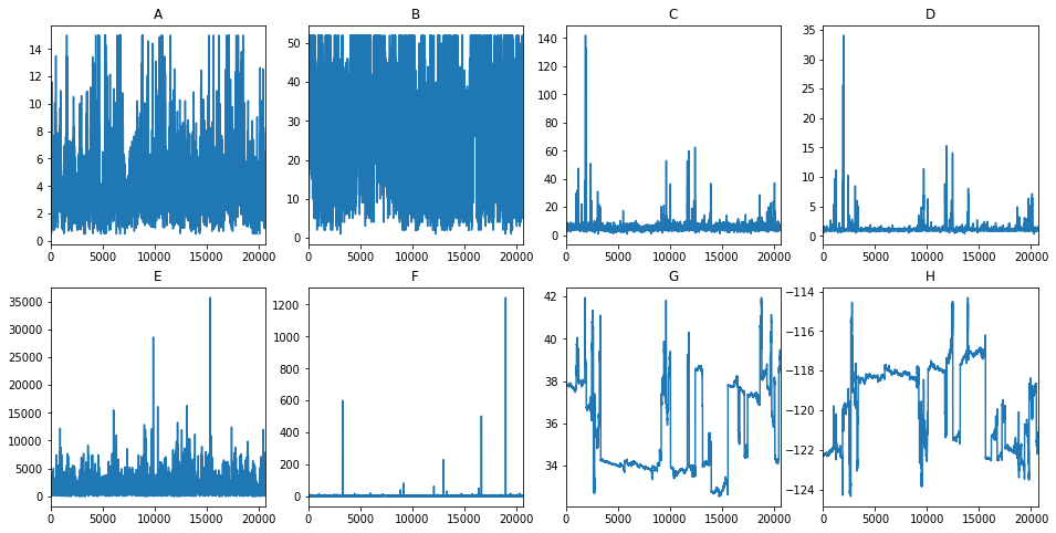
fig, axes = plt.subplots(nrows=2, ncols=4, figsize=(16, 8))

bins = df.shape[0]
df['A'].hist(ax=axes[0, 0], bins=bins);
axes[0, 0].set_title('A');
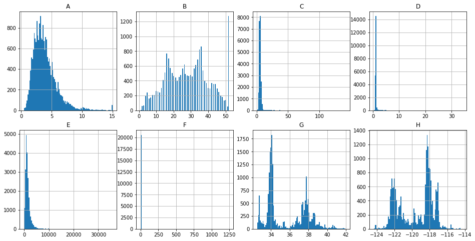
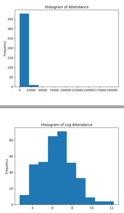
数据如果有偏,可以通过log转换。Estimated Attendance: few missing, right-skewed.
>>> df_train.attendance.isnull().sum()
3

>>> x = df_train.attendance
>>> x.plot(kind='hist',
... title='Histogram of Attendance')

>>> np.log(x).plot(kind='hist',
... title='Histogram of Log Attendance')
可见,转换后接近正态分布。
三、清洗数据
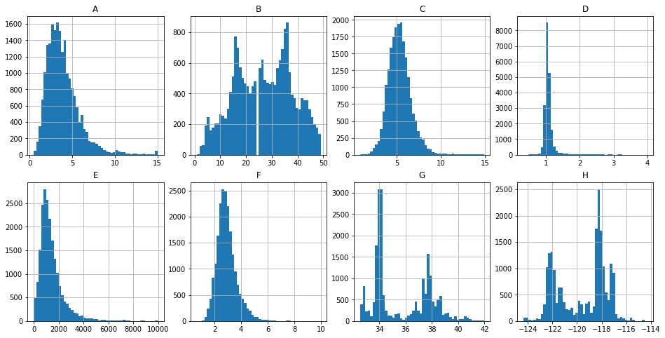
为了去掉极端数据,比如第二行的第二列。
fig, axes = plt.subplots(nrows=2, ncols=4, figsize=(16, 8))
bins = 50

df_f = df['F']
df_f = df_f[df_f < 10]
df_f.hist(ax=axes[1, 1], bins=bins);
axes[0, 0].set_title('A');
L3 - Preprocessing.ipynb
特征预处理
一、原始数据
二、空数据
获取空数据
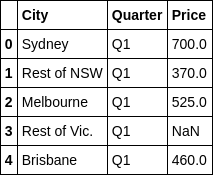
df[pd.isnull(df['Price'])]

index_with_null = df[pd.isnull(df['Price'])].index
统计空数据
df_train数据表 中的 application列,其中的null值的个数统计。
# application_date
appdate_null_ct = df_train.application_date.isnull().sum()
print(appdate_null_ct)  # 3
放弃空数据
Ref: Handling Missing Values in Machine Learning: Part 1
# If axis = 1 then the column will be dropped
df2 = df.dropna(axis=0)

# Will drop all rows that have any missing values.
dataframe.dropna(inplace=True)

# Drop the rows only if all of the values in the row are missing.
dataframe.dropna(how='all',inplace=True)

# Keep only the rows with at least 4 non-na values
dataframe.dropna(thresh=4,inplace=True)
填补空数据
不太好的若干方案。
df2 = df.fillna(0)                       # price value of row 3 is set to 0.0
df2 = df.fillna(method='pad', axis=0)    # The price of row 3 is the same as that of row 2

# Back-fill or forward-fill to propagate next or previous values respectively
#for back fill
dataframe.fillna(method='bfill',inplace=True)
#for forward-fill
dataframe.fillna(method='ffill',inplace=True)
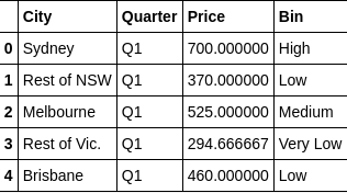
好的方案,求本类别的数据平均值作为替代。
df["Price"] = df.groupby("City").transform(lambda x: x.fillna(x.mean()))

df.ix[index_with_null]  # 之前的index便有了用武之地
三、加标签(二值化)
分区间
讲数值数据分区间,然后加上标签。
# We could label the bins and add new column
df['Bin'] = pd.cut(df['Price'],5,labels=["Very Low","Low","Medium","High","Very High"])

df.head()
与之相对应的 Equal-depth Partitioining,为了使量相等,而让横坐标区间不等。
# Let's check the depth of each bin
df['Bin'] = pd.qcut(df['Price'],5,labels=["Very Low","Low","Medium","High","Very High"])

df.groupby('Bin').size()
加标签后统计
df['Price-Smoothing-mean'] = df.groupby('Bin')['Price'].transform('mean')

df['Price-Smoothing-max']  = df.groupby('Bin')['Price'].transform('max')

四、隐藏数据(去量纲化)
每一列都标准化,之后再加上index,形成新的数据表,隐藏了隐私。
from sklearn import preprocessing

min_max_scaler = preprocessing.StandardScaler()
x_scaled = min_max_scaler.fit_transform(df[df.columns[1:5]]) # we need to remove the first column


df_standard = pd.DataFrame(x_scaled)
df_standard.insert(0, 'City', df.City)
df_standard
特征选择
一、主观判断
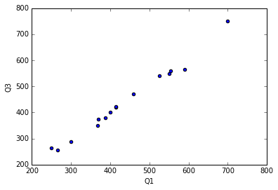
单个图
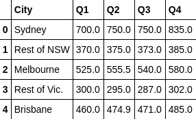
可以看到线性关系。
df.plot.scatter(x='Q1', y='Q3');
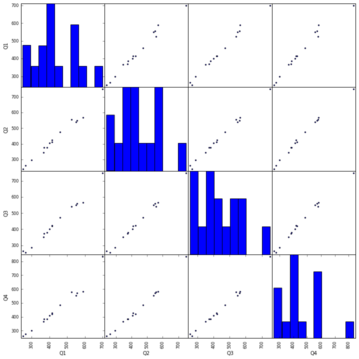
组图
from pandas.plotting import scatter_matrix

scatter_matrix(df, alpha=0.9, figsize=(12, 12), diagonal='hist') # set the diagonal figures to be histograms
二、客观分析
既然是”客观“,建立在判定指标,如下:
3.1 Filter
3.1.1 方差选择法
3.1.2 相关系数法
3.1.3 卡方检验
3.1.4 互信息法
End.

 浙公网安备 33010602011771号