
深度学习面试题37:LSTM Networks原理(Long Short Term Memory networks)
目录
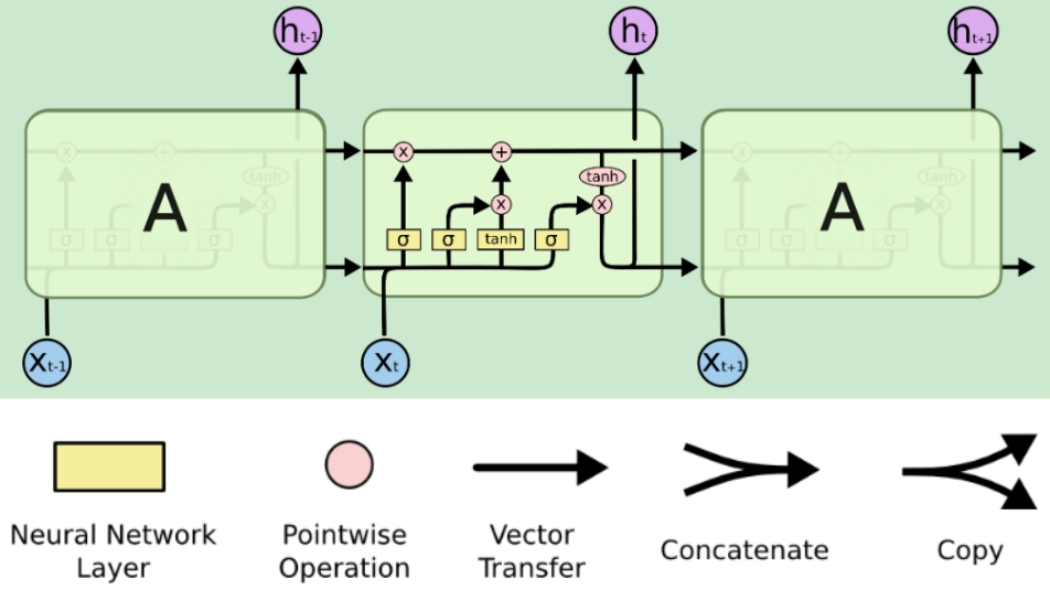
LSTMs网络架构
LSTM的核心思想
遗忘门(Forget gate)
输入门(Input gate)
输出门(Output gate)
LSTMs是如何解决长程依赖问题的?
Peephole是啥
多层LSTM
参考资料
长短期记忆网络通常称为LSTMs,是一种特殊的RNN,能够学习长期依赖关系。他们是由Hochreiter 等人在1997年提出的,在之后的工作中又被很多人精炼和推广。它们对各种各样的问题都非常有效,现在被广泛使用。LSTMs被明确设计为避免长期依赖问题。长时间记忆信息实际上是他们的默认行为,而不是他们努力学习的东西。
|
LSTMs网络架构 |
|
LSTM的核心思想 |
LSTMs的关键是单元状态,即贯穿图表顶部的水平线。细胞的状态有点像传送带。它沿着整个链向下延伸,只有一些小的线性相互作用。很容易让信息不加改变地流动。
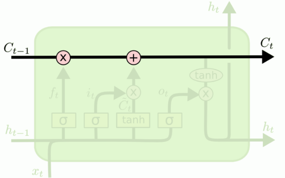
LSTM确实有能力删除或添加信息到细胞状态,由称为门的结构仔细地调节。门是一种选择性地让信息通过的方式。一个LSTM有三个门,以保护和控制单元的状态。
|
遗忘门(Forget gate) |
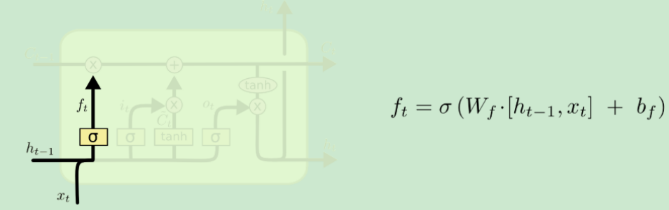
遗忘门会输出一个0到1之间的向量,然后与记忆细胞C做Pointwize的乘法,可以理解为模型正在忘记一些东西。
|
输入门(Input gate) |
有的资料也叫更新门
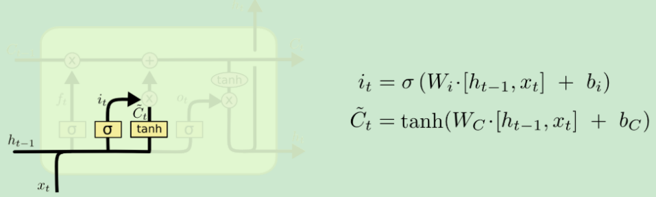
输入门有两条分支,左侧输出一个0到1之间的向量,表示要当前轮多少百分比的信息更新到记忆细胞C上去;右侧表示当前轮提出来的信息。
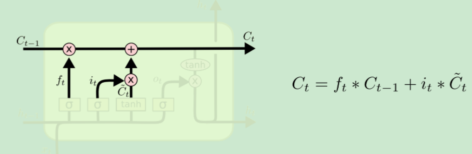
经过遗忘门和输入门之后,记忆细胞便有了一定的变化。
注意LSTM中的记忆细胞只经过遗忘门和输入门,它是不直接经过输出门的。
|
输出门(Output gate) |
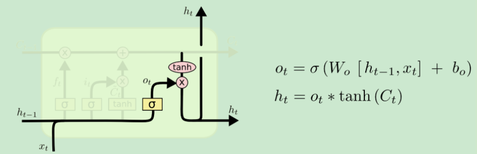
输出门需要接受来自三个方向的输入信息,然后产生两个方向的输出。
三个方向输入的信息分别是:当前时间步的信息、上一个时间步的输出和当前记忆细胞的信息。
两个方向输出的信息分别是:产生当前轮的预测和作为下一个时间步的输入。
|
LSTMs是如何解决长程依赖问题的? |
与简单的RNN网络模型比,LSTMs不是仅仅依靠快速变化的hidden state的信息去产生预测,而是还去考虑记忆细胞C中的信息。
比如有一个有长程依赖的待预测数据:
I grew up in France… I speak fluent ().
当LSTMs读到France后,就把France的信息存在记忆细胞特定的位置上,再经过后面的时间步时,这个France的信息会因为遗忘门的乘法而冲淡,但是要注意,这个冲淡的效果很弱,如果冲刷记忆的效果太强那就和简单的RNN类似了(可能有人要问,要把这个冲刷的强度置为多少呢?答:这是LSTMs自己学出来的),当LSTMs读到fluent时,结合记忆细胞中France的信息,就预测出French的答案。
|
Peephole是啥 |
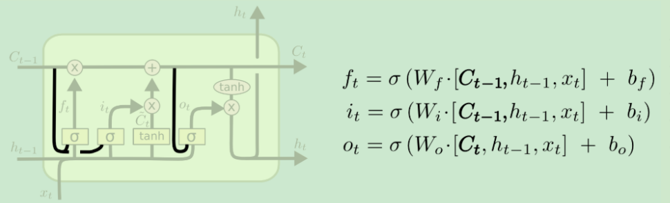
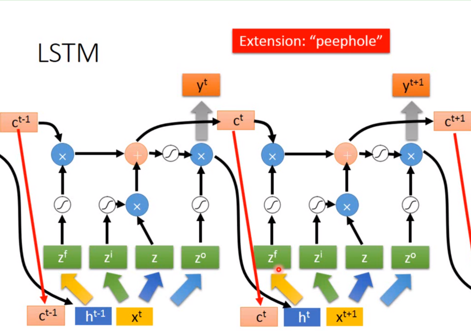
2000年学者Gers & Schmidhuber对LSTMs做了一些变体,peephole如图所示,就是让三个门能利用好记忆细胞里的信息,从而让模型更强。
下图为对应李宏毅老师的结构,是完全一样的。
Pytorch demo


# https://pytorch.org/tutorials/beginner/nlp/sequence_models_tutorial.html?highlight=lstm
# tensorboard --logdir=runs/lstm --host=127.0.0.1
import torch
import torch.nn as nn
import torch.nn.functional as F
import torch.optim as optim

torch.manual_seed(1)


class LSTMTagger(nn.Module):

    def __init__(self, embedding_dim, hidden_dim, vocab_size, tagset_size):
        super(LSTMTagger, self).__init__()
        self.hidden_dim = hidden_dim

        self.word_embeddings = nn.Embedding(vocab_size, embedding_dim)

        # The LSTM takes word embeddings as inputs, and outputs hidden states
        # with dimensionality hidden_dim.
        self.lstm = nn.LSTM(embedding_dim, hidden_dim)

        # The linear layer that maps from hidden state space to tag space
        self.hidden2tag = nn.Linear(hidden_dim, tagset_size)

    def forward(self, sentence):
        embeds = self.word_embeddings(sentence)
        lstm_out, _ = self.lstm(embeds.view(len(sentence), 1, -1))
        tag_space = self.hidden2tag(lstm_out.view(len(sentence), -1))
        tag_scores = F.log_softmax(tag_space, dim=1)
        return tag_scores


def prepare_sequence(seq, to_ix):
    idxs = [to_ix[w] for w in seq]
    return torch.tensor(idxs, dtype=torch.long)


training_data = [
    ("The dog ate the apple".split(), ["DET", "NN", "V", "DET", "NN"]),
    ("Everybody read that book".split(), ["NN", "V", "DET", "NN"])
]
word_to_ix = {}
for sent, tags in training_data:
    for word in sent:
        if word not in word_to_ix:
            word_to_ix[word] = len(word_to_ix)
print(word_to_ix)
tag_to_ix = {"DET": 0, "NN": 1, "V": 2}

# These will usually be more like 32 or 64 dimensional.
# We will keep them small, so we can see how the weights change as we train.
EMBEDDING_DIM = 6
HIDDEN_DIM = 6

model = LSTMTagger(EMBEDDING_DIM, HIDDEN_DIM, len(word_to_ix), len(tag_to_ix))
loss_function = nn.NLLLoss()
optimizer = optim.SGD(model.parameters(), lr=0.1)

# See what the scores are before training
# Note that element i,j of the output is the score for tag j for word i.
# Here we don't need to train, so the code is wrapped in torch.no_grad()

from torch.utils.tensorboard import SummaryWriter
writer = SummaryWriter('../runs/lstm')

with torch.no_grad():
    inputs = prepare_sequence(training_data[0][0], word_to_ix)
    tag_scores = model(inputs)
    writer.add_graph(model, inputs)
    writer.close()

    print(tag_scores)

for epoch in range(300):  # again, normally you would NOT do 300 epochs, it is toy data
    for sentence, tags in training_data:
        # Step 1. Remember that Pytorch accumulates gradients.
        # We need to clear them out before each instance
        model.zero_grad()

        # Step 2. Get our inputs ready for the network, that is, turn them into
        # Tensors of word indices.
        sentence_in = prepare_sequence(sentence, word_to_ix)
        targets = prepare_sequence(tags, tag_to_ix)

        # Step 3. Run our forward pass.
        tag_scores = model(sentence_in)

        # Step 4. Compute the loss, gradients, and update the parameters by
        #  calling optimizer.step()
        loss = loss_function(tag_scores, targets)
        loss.backward()
        optimizer.step()

# See what the scores are after training
with torch.no_grad():
    inputs = prepare_sequence(training_data[0][0], word_to_ix)
    tag_scores = model(inputs)

    # The sentence is "the dog ate the apple".  i,j corresponds to score for tag j
    # for word i. The predicted tag is the maximum scoring tag.
    # Here, we can see the predicted sequence below is 0 1 2 0 1
    # since 0 is index of the maximum value of row 1,
    # 1 is the index of maximum value of row 2, etc.
    # Which is DET NOUN VERB DET NOUN, the correct sequence!
    print(tag_scores)
|
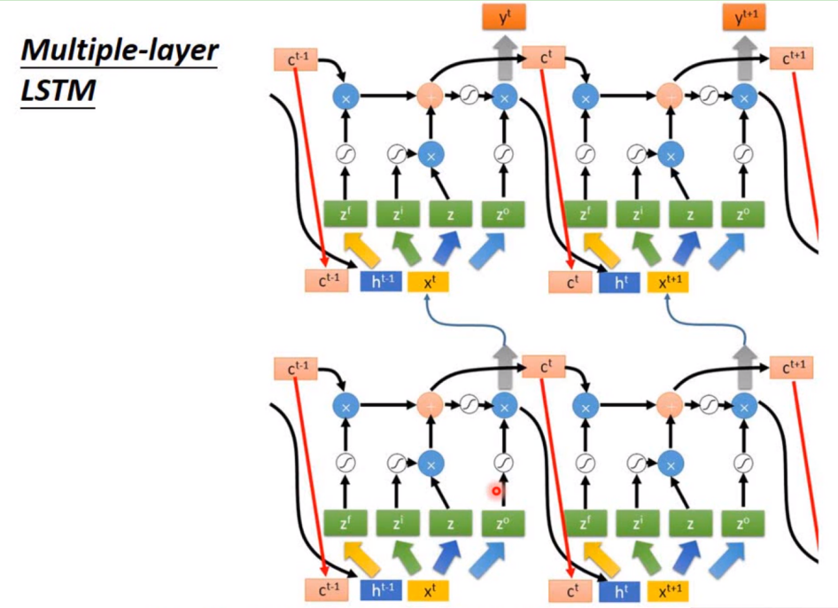
多层LSTM |
和简单的RNN一样,可以叠多层,也可以双向。
|
参考资料 |
https://colah.github.io/posts/2015-08-Understanding-LSTMs/
https://www.bilibili.com/video/BV1JE411g7XF?p=20

 浙公网安备 33010602011771号