【论文阅读】R-CNN:Rich feature hierarchies for accurate object detection and semantic segmentation

Rich feature hierarchies for accurate object detection and semantic segmentation

Ross Girshick Jeff Donahue Trevor Darrell Jitendra Malik

UC Berkeley

rbg,jdonahue,trevor,malikg@eecs.berkeley.edu

Abstract

Object detection performance, as measured on the canonical PASCAL VOC dataset, has plateaued in the last few years. The best-performing methods are complex ensemble systems that typically combine multiple low-level image features with high-level context. In this paper, we propose a simple and scalable detection algorithm that improves mean average precision (mAP) by more than 30% relative to the previous best result on VOC 2012—achieving a mAP of 53.3%. Our approach combines two key insights: (1) one can apply high-capacity convolutional neural networks (CNNs) to bottom-up region proposals in order to localize and segment objects and (2) when labeled training data is scarce, supervised pre-training for an auxiliary task, followed by domain-specific fine-tuning, yields a significant performance boost. Since we combine region proposals with CNNs, we call our method R-CNN: Regions with CNN features. We also compare R-CNN to OverFeat, a recently proposed sliding-window detector based on a similar CNN architecture. We find that R-CNN outperforms OverFeat by a large margin on the 200-class ILSVRC2013 detection dataset. Source code for the complete system is available at http://www.cs.berkeley.edu/rbg/rcnn.

摘要

对象检测性能，例如在典型的PASCAL VOC数据集上测量的结果，在过去几年中已经稳定下来，其中表现最好的方案是将多个低级图像特征与高级语境相结合而组成的复杂系统。在本文中，我们提出了一种简单可扩展的检测算法，其相对于以前的VOC2012数据集的最佳结果，平均精度（mAP）提高了30％以上，达到了53.3％【以前的方法都是传统算法】。我们的方法结合了两个关键点：（1）将大容量（深、复杂）卷积神经网络（CNN）应用于自下而上的候选区域，以便定位和分割对象。（2）当标记的训练数据稀缺时，对辅助任务进行预训练，然后进行域特定的微调，可以显着提升性能【总结起来就是：首先将深度神经网络用于了目标检测和分割，其次是应用了迁移学习】。由于我们将候选区域与CNN相结合，所以我们称我们的方法为R-CNN：具有CNN特征的区域。我们还将R-CNN与OverFeat进行比较，OverFeat是最近提出的基于类似CNN架构的滑动窗口检测器。我们发现R-CNN在ILSVRC2013 200类的检测数据集上大幅超越OverFeat【RCNN的第一版是在OverFeat之前发表的，本文其实是第五版V5，在OverFeat之后发表】。系统的完整源代码在http://www.cs.berkeley.edu/rbg/rcnn。

1. Introduction

Features matter. The last decade of progress on various visual recognition tasks has been based considerably on the use of SIFT [29] and HOG [7]. But if we look at performance on the canonical visual recognition task, PASCAL VOC object detection [15], it is generally acknowledged that progress has been slow during 2010-2012, with small gains obtained by building ensemble systems and employing minor variants of successful methods.

特征很重要。过去的十年中，各种视觉识别任务取得了很大的进步，这取决于SIFT[29]和HOG[7]的使用【建议读者对这两种手工提取的特征进行了解】。但是,如果我们观察典型的视觉识别任务的性能，如PASCAL VOC对象检测[15]，会发现2010-2012年进展缓慢，仅通过组合不同模型和使用已有方法的变体来获得很小的改进。

SIFT and HOG are blockwise orientation histograms, a representation we could associate roughly with complex cells in V1, the first cortical area in the primate visual pathway. But we also know that recognition occurs several stages downstream, which suggests that there might be hierarchical, multi-stage processes for computing features that are even more informative for visual recognition.

SIFT和HOG是块方向直方图，这是一种可以大致与V1中的复合细胞，灵长类动物视觉途径中的第一皮质区域相关联的表示。但是我们也知道识别发生在后续的几个阶段，这表明可能存在层次化，多阶段的计算特征的过程，这些过程对于视觉识别更为有用【由此说明特征提取是一个逐步抽象的过程，需要层次化处理，这正是DCNN所擅长的任务】。

Fukushima’s “neocognitron” [19], a biologically inspired hierarchical and shift-invariant model for pattern recognition, was an early attempt at just such a process. The neocognitron, however, lacked a supervised training algorithm. Building on Rumelhart et al. [33], LeCun et al. [26] showed that stochastic gradient descent via backpropagation was effective for training convolutional neural networks (CNNs), a class of models that extend the neocognitron.

Fukushima的“神经认知机”是一种受生物学启发的分层和偏移不变的模式识别模型，这只是一个早期的尝试。但是，神经认知机缺乏监督训练算法。卷积神经网络（CNN）是一类神经认知机的扩展模型，建立在Rumelhart和LeCun等提出的通过反向传播进行的随机梯度下降的基础之上。

CNNs saw heavy use in the 1990s (e.g., [27]), but then fell out of fashion with the rise of support vector machines. In 2012, Krizhevsky et al. [25] rekindled interest in CNNs by showing substantially higher image classification accuracy on the ImageNet Large Scale Visual Recognition Challenge (ILSVRC) [9, 10]. Their success resulted from training a large CNN on 1.2 million labeled images, together with a few twists on LeCun’s CNN (e.g., max(x, 0) rectifying non-linearities and “dropout” regularization).

CNN在20世纪90年代有广泛的使用（例如27），但是随着支持向量机的兴起，CNN已经逐渐淡出了公众视野。 2012年，Krizhevsky等在ImageNet大型视觉识别挑战（ILSVRC）上显示出更高的图像分类准确度，重新唤起了人们对CNN的兴趣【AlexNet这个模型很重要，简单但很经典，建议细读****】。他们通过使用大型CNN训练120万张带标记图像而，以及对LeCun的CNN的一些改进（例如，max(x，0)修正线性单元和“Dropout”正规化）而成功。

The significance of the ImageNet result was vigorously debated during the ILSVRC 2012 workshop. The central issue can be distilled to the following: To what extent do the CNN classification results on ImageNet generalize to object detection results on the PASCAL VOC Challenge?

ImageNet结果的意义在ILSVRC 2012研讨会期间大有争议。中心问题可以归结为：CNN对ImageNet的分类结果在多大程度上可以泛化为PASCAL VOC目标检测挑战赛的结果？【简单点说就是图像分类训练的模型对于目标检测类任务有没有帮助，因为图像分类任务的数据集十分丰富，而用于检测任务的数据集却相对较少】

We answer this question by bridging the gap between image classification and object detection. This paper is the first to show that a CNN can lead to dramatically higher object detection performance on PASCAL VOC as compared to systems based on simpler HOG-like features. To achieve this result, we focused on two problems: localizing objects with a deep network and training a high-capacity model with only a small quantity of annotated detection data.

我们通过弥合图像分类和对象检测之间的差距来回答这个问题。本文最先提出：与基于更简单的HOG类特征的系统相比，CNN可以显著提高PASCAL VOC的目标检测性能。为了实现这一结果，我们主要关注两个问题：使用深度网络定位目标，并只使用少量带标记的检测数据训练高容量模型。

Unlike image classification, detection requires localizing (likely many) objects within an image. One approach frames localization as a regression problem. However, work from Szegedy et al. [38], concurrent with our own, indicates that this strategy may not fare well in practice (they report a map of 30.5% on VOC 2007 compared to the 58.5% achieved by our method). An alternative is to build a sliding-window detector. CNNs have been used in this way for at least two decades, typically on constrained object categories, such as faces [32, 40] and pedestrians [35]. In order to maintain high spatial resolution, these CNNs typically only have two convolutional and pooling layers. We also considered adopting a sliding-window approach. However, units high up in our network, which has five convolutional layers, have very large receptive fields (195 × 195 pixels) and strides (32×32 pixels) in the input image, which makes precise localization within the sliding-window paradigm an open technical challenge.

与图像分类不同，检测需要在图像中定位（可能是许多）目标。一种方法是将定位作为回归问题。然而，Szeged等人[38]与我们的工作表明这种策略在实践中可能不会很好（他们在VOC 2007年的map为30.5％，而我们的方法达到了58.5％）。另一种方法是构建一个滑动窗口检测器。 CNN已经以这种方式使用了至少二十年，通常是在限定的物体类别上，如面部和行人。为了保持高空间分辨率，这些CNN通常只有两个卷积和池化层。我们也考虑了采用滑动窗口方法。然而，在我们的网络中，具有五个卷积层的单元在输入图像中具有非常大的接收域（195×195像素）和步长（32×32像素）【如何根据卷积步长的不同组合方式来计算感受野的大小很重要，建议熟知】，这使得在滑动窗口内的精确定位成为公开的技术挑战。

Instead, we solve the CNN localization problem by operating within the “recognition using regions” paradigm [21], which has been successful for both object detection [39] and semantic segmentation [5]. At test time, our method generates around 2000 category-independent region proposals for the input image, extracts a fixed-length feature vector from each proposal using a CNN, and then classifies each region with category-specific linear SVMs. We use a simple technique (affine image warping) to compute a fixed-size CNN input from each region proposal, regardless of the region’s shape. Figure 1 presents an overview of our method and highlights some of our results. Since our system combines region proposals with CNNs, we dub the method R-CNN: Regions with CNN features.

相反，我们通过“基于区域提案的识别”范式来解决CNN的定位问题，这已经成功实现了目标检测和语义分割。在测试阶段，我们的方法为输入图像生成大约2000个类别无关的候选区域，使用CNN从每个提案中提取固定长度的特征向量，然后对每个区域进行类别特定的线性SVM分类。我们使用简单的技术（图像仿射变换，就是直接拉伸）来将每个区域提案拉伸到固定大小作为CNN的输入，而不管区域的形状。图1是我们方法的概述，彰显了我们的一些成果。由于我们的系统将区域提案与CNN相结合，所以我们将方法命名为R-CNN：具有CNN特征的区域。

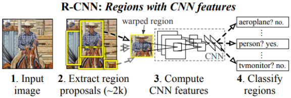
Figure 1: Object detection system overview. Our system (1) takes an input image, (2) extracts around 2000 bottom-up region proposals, (3) computes features for each proposal using a large convolutional neural network (CNN), and then (4) classifies each region using class-specific linear SVMs. R-CNN achieves a mean average precision (map) of 53.7% on PASCAL VOC 2010. For comparison, [39] reports 35.1% map using the same region proposals, but with a spatial pyramid and bag-of-visual-words approach. The popular deformable part models perform at 33.4%. On the 200-class ILSVRC2013 detection dataset, R-CNN’s map is 31.4%, a large improvement over OverFeat [34], which had the previous best result at 24.3%.

图1：对象检测系统概述。我们的系统（1）输入一张图像，（2）提取约2000个自下而上的区域提案，（3）使用深度卷积神经网络（CNN）计算每个提案的特征，然后（4）使用类别特定的线性SVM对每个提案分类。 R-CNN在PASCAL VOC 2010中实现了53.7％的平均精度（map）。相较之下，[39]使用了相同的区域提案，但是使用了空间金字塔和bag-of-visual-words方法，达到了35.1％的map。主流的可变形部件模型为33.4％。在200类的ILSVRC2013检测数据集上，R-CNN的map为31.4％，超过OverFeat很多，OverFeat最佳结果为24.3％。）

In this updated version of this paper, we provide a head-to-head comparison of R-CNN and the recently proposed OverFeat [34] detection system by running R-CNN on the 200-class ILSVRC2013 detection dataset. OverFeat uses a sliding-window CNN for detection and until now was the best performing method on ILSVRC2013 detection. We show that R-CNN significantly outperforms OverFeat, with a map of 31.4% versus 24.3%

在本文的更新版本中，我们让R-CNN和最近提出的OverFeat检测系统在200类的ILSVRC2013检测数据集上运行，提供详细的比较结果。OverFeat使用滑动窗口CNN进行检测，是目前在ILSVRC2013检测中性能最好的方法。我们的R-CNN明显优于OverFeat，map为31.4％，而OverFeat是24.3％。

A second challenge faced in detection is that labeled data is scarce and the amount currently available is insufficient for training a large CNN. The conventional solution to this problem is to use unsupervised pre-training, followed by supervised fine-tuning (e.g., [35]). The second principle contribution of this paper is to show thatsupervised pre-training on a large auxiliary dataset (ILSVRC), followed by domainspecific fine-tuning on a small dataset (PASCAL), is an effective paradigm for learning high-capacity CNNs when data is scarce. In our experiments, fine-tuning for detection improves map performance by 8 percentage points. After fine-tuning, our system achieves a map of 54% on VOC 2010 compared to 33% for the highly-tuned, HOG-based deformable part model (DPM) [17, 20]. We also point readers to contemporaneous work by Donahue et al. [12], who show that Krizhevsky’s CNN can be used (without finetuning) as a blackbox feature extractor, yielding excellent performance on several recognition tasks including scene classification, fine-grained sub-categorization, and domain adaptation.

检测面临的第二个挑战是标记的数据很少且目前可用的数量不足以训练大型CNN。这个问题的常规解决方案是使用无监督的预训练，然后进行辅助微调（见35）。本文的第二个主要贡献是在大型辅助数据集(ILSVRC)上进行监督预训练，然后对小数据集(PASCAL)进行域特定的微调，这是在数据稀缺时训练高容量CNN模型的有效范例。在我们的实验中，微调将检测的map性能提高了8个百分点。微调后，我们的系统在VOC 2010上实现了54％的map，而高度优化的基于HOG的可变形部件模型(DPM)为33％。同时，Donahue等人进行的工作[12]表明可以使用Krizhevsky的CNN（无需微调）作为黑盒特征提取器，在多个识别任务（包括场景分类，细粒度子分类和领域适应）中表现出色。

Our system is also quite efficient. The only class-specific computations are a reasonably small matrix-vector product and greedy non-maximum suppression. This computational property follows from features that are shared across all categories and that are also two orders of magnitude lower dimensional than previously used region features (cf. [39]).

我们的系统也很有效率。唯一的类特定计算是相当小的矩阵向量乘积和基于贪心规则的非极大值抑制【在进行SVM分类的时候需要用到矩阵乘法，每个类别单独计算，不能共享，后面的NMS也是不能共享计算】。这种计算属性来自于跨所有样本类别共享的特征，并且比以前使用的区域特征维度还低两个数量级(这个怎么理解呢？)（参见39）。

Understanding the failure modes of our approach is also critical for improving it, and so we report results from the detection analysis tool of Hoiem et al. [23]. As an immediate consequence of this analysis, we demonstrate that a simple bounding-box regression method significantly reduces mislocalizations, which are the dominant error mode.

分析我们方法的不足之处对于改进模型也是至关重要的，因此我们给出了由Hoiem等人提出的检测分析工具的结果。通过****这一分析，我们证明了一种简单的边界回归方法显著地减少了定位误差，这是主要的误差模式。

Before developing technical details, we note that because R-CNN operates on regions it is natural to extend it to the task of semantic segmentation. With minor modifications, we also achieve competitive results on the PASCAL VOC segmentation task, with an average segmentation accuracy of 47.9% on the VOC 2011 test set.

在发掘技术细节之前，我们注意到：由于R-CNN在区域上运行，将其扩展到语义分割的任务就很自然。经过少量的修改，我们也在PASCAL VOC分割任务中取得了有竞争力的成果，VOC 2011测试集的平均分割精度为47.9％。

2. Object detection with R-CNN

Our object detection system consists of three modules. The first generates category-independent region proposals. These proposals define the set of candidate detections available to our detector. The second module is a large convolutional neural network that extracts a fixed-length feature vector from each region. The third module is a set of classspecific linear SVMs. In this section, we present our design decisions for each module, describe their test-time usage, detail how their parameters are learned, and show detection results on PASCAL VOC 2010-12 and on ILSVRC2013.

我们的目标检测系统由三个模块组成。第一个生成类别无关区域提案。这些提案定义了可用于我们的检测器的候选检测集。第二个模块是从每个区域提取固定长度特征向量的大型卷积神经网络。第三个模块是一组特定类别的线性SVM。在本节中，我们介绍每个模块的设计思路，描述其测试时使用情况，详细介绍其参数的学习方式，并给出在PASCAL VOC 2010-12和ILSVRC2013上的检测结果。

2.1. Module design

Region proposals. A variety of recent papers offer methods for generating category-independent region proposals. Examples include: objectness [1], selective search [39], category-independent object proposals [14], constrained parametric min-cuts (CPMC) [5], multi-scale combinatorial grouping [3], and Ciresan et al. [6], who detect mitotic cells by applying a CNN to regularly-spaced square crops, which are a special case of region proposals. While R-CNN is agnostic to the particular region proposal method, we use selective search to enable a controlled comparison with prior detection work (e.g., [39, 41]).

*区域提案。*最近的各种论文提供了生成类别无关区域提案的方法。例子包括：objectness [1]，选择性搜索[39]，类别无关对象提议[14]，约束参数最小化(CPMC)[5]【这些区域提案算法基本上是基于图像的纹理、轮廓、色彩等特征的】，多尺度组合分组[3]和Ciresan等提出的[6]通过将CNN应用于特定间隔的方块来检测有丝分裂细胞，这是区域提案的特殊情况。具体的区域提案方法对于R-CNN是透明的，但我们使用选择性搜索以便于与先前检测工作的对照比较（例如39,41）。

Feature extraction. We extract a 4096-dimensional feature vector from each region proposal using the Caffe [24] implementation of the CNN described by Krizhevsky et al. [25]. Features are computed by forward propagating a mean-subtracted 227 × 227 RGB image through five convolutional layers and two fully connected layers. We refer readers to [24, 25] for more network architecture details.

*特征提取。*我们使用Krizhevsky等人提出的CNN的Caffe[24]实现，从每个区域提案中提取4096维特征向量。将227×227分辨率的RGB图像减去像素平均值后通过五个卷积层和两个全连接层向前传播来计算特征。可以参考24，25以获得更多的网络架构细节【建议参考文章实现一下】。

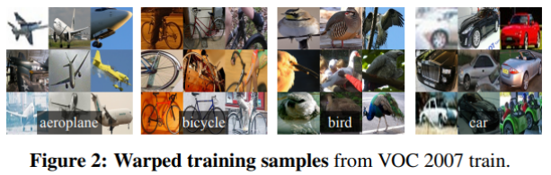
In order to compute features for a region proposal, we must first convert the image data in that region into a form that is compatible with the CNN (its architecture requires inputs of a fixed 227 × 227 pixel size). Of the many possible transformations of our arbitrary-shaped regions, we opt for the simplest. Regardless of the size or aspect ratio of the candidate region, we warp all pixels in a tight bounding box around it to the required size. Prior to warping, we dilate the tight bounding box so that at the warped size there are exactly p pixels of warped image context around the original box (we use p = 16). Figure 2 shows a random sampling of warped training regions. Alternatives to warping are discussed in Appendix A.

为了计算区域提案的特征，我们必须首先将该区域中的图像数据转换为与CNN兼容的格式（其架构需要固定227×227像素大小的输入）。在许多可能的针对任意形状区域的变换中，我们选择最简单的。不管候选区域的大小或横纵比如何，我们将整个区域不保持横纵比缩放到所需的大小。在缩放之前，我们扩大了被缩放的区域，使得在缩放后，原始区域边界到现有区域边界宽度为p像素（我们使用p = 16）。图2显示了变形训练区域的随机抽样。变形的替代方案在附录A中讨论【就是描述了如何将候选区域拉升到227X227的大小作为网络的输入以便提取CNN的4096维特征，具体描述可以参考博客图文理解】。

2.2. Test-time detection

At test time, we run selective search on the test image to extract around 2000 region proposals (we use selective search’s “fast mode” in all experiments). We warp each proposal and forward propagate it through the CNN in order to compute features. Then, for each class, we score each extracted feature vector using the SVM trained for that class. Given all scored regions in an image, we apply a greedy non-maximum suppression (for each class independently) that rejects a region if it has an intersection over union (IoU) overlap with a higher scoring selected region larger than a learned threshold.

在测试时，我们对测试图像进行选择性搜索，以提取大约2000个区域提案（我们在所有实验中使用选择性搜索的“快速模式”）。然后缩放每个区域，并通过CNN向前传播，以计算特征。最后，对于每个类，我们使用针对该类训练的SVM来对每个提取的特征向量进行评分。给定图像中的所有区域的得分后，我们应用贪婪非极大值抑制（每个类别独立进行），在训练时学习一个阈值，如果其与得分较高的区域的重叠部分(IoU)高于这个阈值，则丢弃这个区域。

Run-time analysis. Two properties make detection efficient. First, all CNN parameters are shared across all categories. Second, the feature vectors computed by the CNN are low-dimensional when compared to other common approaches, such as spatial pyramids with bag-of-visual-word encodings. The features used in the UVA detection system [39], for example, are two orders of magnitude larger than ours (360k vs. 4k-dimensional).

*性能分析。*两种性质使检测效率高。首先，所有CNN参数都在所有类别中共享【作者这意思是说所有的候选区域都是通过同一个CNN模型提取特征】。其次，与其他常见方法比较，由CNN计算出的特征向量是低维度的，例如具有空间金字塔和bag-of-visual-word的方法。UVA检测系统39中使用的特征比我们（维度，360k对比4k）大两个数量级。

The result of such sharing is that the time spent computing region proposals and features (13s/image on a GPU or 53s/image on a CPU) is amortized over all classes. The only class-specific computations are dot products between features and SVM weights and non-maximum suppression. In practice, all dot products for an image are batched into a single matrix-matrix product. The feature matrix is typically 2000×4096 and the SVM weight matrix is 4096×N, where N is the number of classes.

这种共享的结果是计算区域建议和特征（GPU上的13秒/图像或CPU上的53秒/图像）的时间在所有类别上进行摊销。唯一的类特定计算是特征与SVM权重的点积和非极大值抑制。在实践中，图像的所有点积运算都被整合为单个矩阵与矩阵的相乘。特征矩阵通常为2000×4096，SVM权重矩阵为4096×N，其中N为类别数。

This analysis shows that R-CNN can scale to thousands of object classes without resorting to approximate techniques, such as hashing. Even if there were 100k classes, the resulting matrix multiplication takes only 10 seconds on a modern multi-core CPU. This efficiency is not merely the result of using region proposals and shared features. The UVA system, due to its high-dimensional features, would be two orders of magnitude slower while requiring 134GB of memory just to store 100k linear predictors, compared to just 1.5GB for our lower-dimensional features.

如上的分析表明，R-CNN可以扩展到数千个类，而不需要使用如散列这样的技术。即使有10万个类，在现代多核CPU上产生的矩阵乘法只需10秒。这种效率不仅仅是使用区域提案和共享特征的结果。由于其高维度特征，UVA系统的速度将会降低两个数量级，并且需要134GB的内存来存储10万个线性预测器。而对于低维度特征而言，仅需要1.5GB内存【这段内容分析好牵强】。

It is also interesting to contrast R-CNN with the recent work from Dean et al. on scalable detection using DPMs and hashing [8]. They report a map of around 16% on VOC 2007 at a run-time of 5 minutes per image when introducing 10k distractor classes. With our approach, 10k detectors can run in about a minute on a CPU, and because no approximations are made map would remain at 59% (Section 3.2).

将R-CNN与Dean等人最近的工作对比也是有趣的。使用DPM和散列的可扩展检测。在引入1万个干扰类的情况下，每个图像的运行时间为5分钟，其在VOC 2007上的map约为16％。通过我们的方法，1万个检测器可以在CPU上运行大约一分钟，而且由于没有近似值，可以使map保持在59％（见消融研究）。

2.3. Training

Supervised pre-training. We discriminatively pre-trained the CNN on a large auxiliary dataset (ILSVRC2012 classification) using image-level annotations only (bounding box labels are not available for this data). Pre-training was performed using the open source Caffe CNN library [24]. In brief, our CNN nearly matches the performance of Krizhevsky et al. [25], obtaining a top-1 error rate 2.2 percentage points higher on the ILSVRC2012 classification validation set. This discrepancy is due to simplifications in the training process.

*监督预训练。*我们仅通过使用图像级标记（此数据没有检测框标记）的大型辅助数据集（ILSVRC2012分类数据集）来区分性地对CNN进行预训练。使用开源的Caffe CNN库进行预训练。简而言之，我们的CNN几乎符合Krizhevsky等人的论文中的表现，ILSVRC2012分类验证集获得的top-1错误率高出2.2个百分点。这种差异是由于训练过程中的简化造成的【首先大致复现了AlexNet分类网络的性能】。

Domain-specific fine-tuning. To adapt our CNN to the new task (detection) and the new domain (warped proposal windows), we continue stochastic gradient descent (SGD) training of the CNN parameters using only warped region proposals. Aside from replacing the CNN’s ImageNet specific 1000-way classification layer with a randomly initialized (N + 1)-way classification layer (where N is the number of object classes, plus 1 for background), the CNN architecture is unchanged. For VOC, N = 20 and for ILSVRC2013, N = 200. We treat all region proposals with ≥ 0.5 IoU overlap with a ground-truth box as positives for that box’s class and the rest as negatives. We start SGD at a learning rate of 0.001 (1/10th of the initial pre-training rate), which allows fine-tuning to make progress while not clobbering the initialization. In each SGD iteration, we uniformly sample 32 positive windows (over all classes) and 96 background windows to construct a mini-batch of size 128. We bias the sampling towards positive windows because they are extremely rare compared to background.

*域特定的微调。*为了使CNN适应新任务（检测）和新域（缩放的提案窗口），我们仅使用缩放后的区域提案继续进行CNN参数的随机梯度下降(SGD)训练。除了用随机初始化的(N + 1)路分类层（其中N是类别数，加1为背景）替换CNN的ImageNet特有的1000路分类层，CNN架构不变【简单介绍了一下如何更改网络】。对于VOC，N = 20，对于ILSVRC2013，N = 200。我们将所有区域提案与检测框真值IoU ≥0.5的区域作为正样本，其余的作为负样本。我们以0.001（初始学习率的1/10）的学习率开始SGD，这样可以在不破坏初始化的情况下进行微调。在每个SGD迭代中，我们从所有类别中统一采样32个正样本和96个负样本，以构建大小为128的小批量。采样的正样本较少是因为它们与背景相比非常罕见。

Object category classifiers. Consider training a binary classifier to detect cars. It’s clear that an image region tightly enclosing a car should be a positive example. Similarly, it’s clear that a background region, which has nothing to do with cars, should be a negative example. Less clear is how to label a region that partially overlaps a car. We resolve this issue with an IoU overlap threshold, below which regions are defined as negatives. The overlap threshold, 0.3, was selected by a grid search over {0, 0.1, . . . , 0.5} on a validation set. We found that selecting this threshold carefully is important. Setting it to 0.5, as in [39], decreased map by 5 points. Similarly, setting it to 0 decreased map by 4 points. Positive examples are defined simply to be the ground-truth bounding boxes for each class.

*目标类别分类器。*考虑训练二分类器来检测汽车。很明显，紧紧围绕汽车的图像区域应该是一个正样例，一个与汽车无关的背景区域应该是一个负样本。较不清楚的是如何标注部分重叠汽车的区域。我们用IoU重叠阈值来解决这个问题，在这个阈值以下的区域被定义为负样本。重叠阈值0.3是通过在验证集上尝试了0,0.1,…,0.50,0.1,…,0.5的不同阈值选择出来的。我们发现选择这个阈值是很重要的。将其设置为0.5，如39，map会降低5个点。同样，将其设置为0会将map降低4个点。正样本被简单地定义为每个类的检测框真值。

Once features are extracted and training labels are applied, we optimize one linear SVM per class. Since the training data is too large to fit in memory, we adopt the standard hard negative mining method [17, 37]. Hard negative mining converges quickly and in practice map stops increasing after only a single pass over all images.

一旦提取了特征并有了训练标签，我们就可以优化每类线性SVM。由于训练数据太大内存不够，我们采用标准的难分样本挖掘方法[17,37]。难分样本挖掘可以快速收敛，实际上所有图像遍历一遍，map就停止增长了。

In Appendix B we discuss why the positive and negative examples are defined differently in fine-tuning versus SVM training. We also discuss the trade-offs involved in training detection SVMs rather than simply using the outputs from the final softmax layer of the fine-tuned CNN.

在附录B中，我们将讨论为什么在微调与SVM训练中，正样本和负样本的数量不同。我们还讨论了涉及训练检测SVM的权衡，而不是简单地使用微调CNN的最终softmax层的输出。

2.4. Results on PASCAL VOC 2010-12

Following the PASCAL VOC best practices [15], we validated all design decisions and hyperparameters on the VOC 2007 dataset (Section 3.2). For final results on the VOC 2010-12 datasets, we fine-tuned the CNN on VOC 2012 train and optimized our detection SVMs on VOC 2012 trainval. We submitted test results to the evaluation server only once for each of the two major algorithm variants (with and without bounding-box regression).

根据PASCAL VOC最佳实践15，我们在VOC 2007数据集上验证了所有设计和超参数（见消融研究）。对于VOC 2010-12数据集的最终结果，我们对VOC 2012 train上对CNN进行了微调，并在VOC 2012 trainval上优化检测SVM。我们将测试结果提交给评估服务器，对于两种主要算法变体（带有和不带有检测框回归）的每一种，都只提交一次。

Table 1 shows complete results on VOC 2010. We compare our method against four strong baselines, including SegDPM [18], which combines DPM detectors with the output of a semantic segmentation system [4] and uses additional inter-detector context and image-classifier rescoring. The most germane comparison is to the UVA system from Uijlings et al. [39], since our systems use the same region proposal algorithm. To classify regions, their method builds a four-level spatial pyramid and populates it with densely sampled SIFT, Extended Opponent SIFT, and RGBSIFT descriptors, each vector quantized with 4000-word codebooks. Classification is performed with a histogram intersection kernel SVM. Compared to their multi-feature, non-linear kernel SVM approach, we achieve a large improvement in map, from 35.1% to 53.7% map, while also being much faster (Section 2.2). Our method achieves similar performance (53.3% map) on VOC 2011/12 test.

表1显示了VOC2010的完整结果。我们与其它四种很优秀的方法进行了比较，包括SegDPM，它将DPM检测器与语义分割系统的输出相结合，并使用了像语境和图像类别重排的内部分类器。最具可比性的是Uijlings等人的UVA系统，因为我们的系统使用相同的区域提案算法。为了对区域进行分类，他们的方法构建了一个四级空间金字塔，并用密集采样的SIFT(（扩展对准SIFT和RGB-SIFT描述符，每个矢量用4000字的码本量化），使用直方图交叉核心SVM进行分类。与其多特征非线性内核SVM方法相比，我们将map从35.1％提高到了53.7％，同时也快得多（见测试）。我们的方法在VOC 2011/12测试中实现了接近的性能（53.3％的map）。

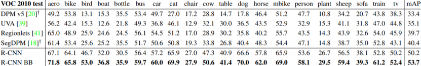
Table 1: Detection average precision (%) on VOC 2010 test. R-CNN is most directly comparable to UVA and Regionlets since all methods use selective search region proposals. Bounding-box regression (BB) is described in Section C. At publication time, SegDPM was the top-performer on the PASCAL VOC leaderboard. †DPM and SegDPM use context rescoring not used by the other methods.

表1：（VOC 2010测试的平均检测精度（％）。 R-CNN与UVA和Regionlets最相似，因为所有方法都使用选择性搜索区域提案。检测框回归（BB）在附录C中描述。在本文发布时，SegDPM是PASCAL VOC排行榜中表现最好的方法。 †DPM和SegDPM使用上下文重排，其他方法未使用）

2.5. Results on ILSVRC2013 detection

We ran R-CNN on the 200-class ILSVRC2013 detection dataset using the same system hyperparameters that we used for PASCAL VOC. We followed the same protocol of submitting test results to the ILSVRC2013 evaluation server only twice, once with and once without bounding-box regression.

我们使用与PASCAL VOC相同的系统超参数，在200类的ILSVRC2013检测数据集上运行R-CNN。我们遵循相同的原则，仅提交测试结果给ILSVRC2013评估服务器两次，一次有边界框回归，一次没有。

Figure 3 compares R-CNN to the entries in the ILSVRC 2013 competition and to the post-competition OverFeat result [34]. R-CNN achieves a map of 31.4%, which is significantly ahead of the second-best result of 24.3% from OverFeat. To give a sense of the AP distribution over classes, box plots are also presented and a table of perclass APs follows at the end of the paper in Table 8. Most of the competing submissions (OverFeat, NEC-MU, UvAEuvision, Toronto A, and UIUC-IFP) used convolutional neural networks, indicating that there is significant nuance in how CNNs can be applied to object detection, leading to greatly varying outcomes.

图3比较了R-CNN与ILSVRC 2013竞赛中的参赛作品以及赛后OverFeat得结果[34]。 R-CNN的map达到31.4％，远远高于OverFeat的24.3％的第二好成绩。为了了解类别上的AP分布情况，还提供了箱形图，并在表8的结尾处列出了每类AP的表格。提交的大多数竞争性结果（OverFeat，NEC-MU，UvAEuvision，Toronto A，和UIUC-IFP）都使用卷积神经网络，表明CNN如何应用于物体检测存在显着的细微差别，导致结果差异很大。

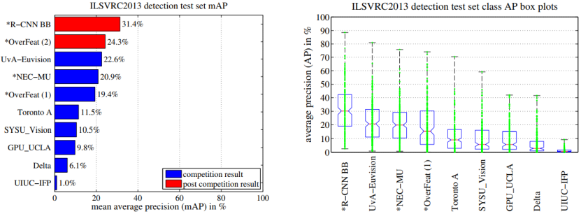
Figure 3: (Left) Mean average precision on the ILSVRC2013 detection test set. Methods preceeded by * use outside training data (images and labels from the ILSVRC classification dataset in all cases). (Right) Box plots for the 200 average precision values per method. A box plot for the post-competition OverFeat result is not shown because per-class APs are not yet available (per-class APs for R-CNN are in Table 8 and also included in the tech report source uploaded to arXiv.org; see R-CNN-ILSVRC2013-APs.txt). The red line marks the median AP, the box bottom and top are the 25th and 75th percentiles. The whiskers extend to the min and max AP of each method. Each AP is plotted as a green dot over the whiskers (best viewed digitally with zoom).

图3：（左）ILSVRC2013检测测试集的平均精度。方法之前有符号*表示使用外部训练数据（都使用ILSVRC分类数据集的图像和标签）。（右）200个类map的箱形图方法。没有显示赛后OverFeat结果的方框图，因为每类AP尚不可用（R-CNN每类的AP为见表8，也包含在上传到arXiv.org的技术报告中; 见R-CNN-ILSVRC2013-APs.txt）。这红色线标记中位数AP，方框底部和顶部是第25和第75百分位数。虚线延伸到每个的最小和最大AP方法。每个AP在虚线上绘制为绿点（最好以数字方式使用缩放查看）。

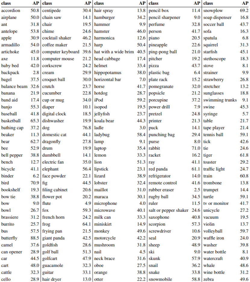
Table 8: Per-class average precision (%) on the ILSVRC2013 detection test set.

In Section 4, we give an overview of the ILSVRC2013 detection dataset and provide details about choices that we made when running R-CNN on it.

在第4节中，我们概述了ILSVRC2013检测数据集，并提供了有关在其上运行R-CNN时所做选择的详细信息。

3. Visualization, ablation, and modes of error

3.1. Visualizing learned features

First-layer filters can be visualized directly and are easy to understand [25]. They capture oriented edges and opponent colors. Understanding the subsequent layers is more challenging. Zeiler and Fergus present a visually attractive deconvolutional approach in [42]. We propose a simple (and complementary) non-parametric method that directly shows what the network learned.

第一层卷积核可以直观可视化，易于理解。它们捕获定向边缘和相对颜色。了解后续层次更具挑战性。 Zeiler和Fergus在提出了一种有视觉吸引力的反卷积方法。我们提出一个简单（和补充）非参数方法，直接显示网络学到的内容。

The idea is to single out a particular unit (feature) in the network and use it as if it were an object detector in its own right. That is, we compute the unit’s activations on a large set of held-out region proposals (about 10 million), sort the proposals from highest to lowest activation, perform nonmaximum suppression, and then display the top-scoring regions. Our method lets the selected unit “speak for itself” by showing exactly which inputs it fires on. We avoid averaging in order to see different visual modes and gain insight into the invariances computed by the unit.

这个想法是在网络中列出一个特定的单元（特征），并将其用作它自己的目标检测器。也就是说，我们在大量的区域提案（约1000万【每张图像约2000个候选区域】）中计算这个单元的激活，将提案按激活从大到小排序，然后执行非极大值抑制，然后显示激活最大的提案。通过准确显示它激活了哪些输入，我们的方法让所选单元“自己说话”。我们避免平均，以看到不同的视觉模式，并深入了解这个单元计算的不变性。

We visualize units from layer pool5 , which is the max pooled output of the network’s fifth and final convolutional layer. The pool5 feature map is 6 × 6 × 256 = 9216- dimensional. Ignoring boundary effects, each pool5 unit has a receptive field of 195×195 pixels in the original 227×227 pixel input. A central pool5 unit has a nearly global view, while one near the edge has a smaller, clipped support.

我们可以看到来自pool5的单元，这是网络第五，也是最终卷积层的最大池化输出。pool5的特征图维度是6×6×256=9216。忽略边界效应，每个pool5单元在原始227×227像素输入中具有195×195像素的感受野。位于中央的pool5单元具有几乎全局的视野，而靠近边缘的则有一个较小的裁剪的视野。

Each row in Figure 4 displays the top 16 activations for a pool5 unit from a CNN that we fine-tuned on VOC 2007 trainval. Six of the 256 functionally unique units are visualized (Appendix D includes more). These units were selected to show a representative sample of what the network learns. In the second row, we see a unit that fires on dog faces and dot arrays. The unit corresponding to the third row is a red blob detector. There are also detectors for human faces and more abstract patterns such as text and triangular structures with windows. The network appears to learn a representation that combines a small number of class-tuned features together with a distributed representation of shape, texture, color, and material properties. The subsequent fully connected layer fc6 has the ability to model a large set of compositions of these rich features.

图4中的每一行都显示了在VOC 2007 trainval上进行微调的CNN中的pool5单元的前16个最大激活的区域【也就是置信度最高得几个？】，包括256个功能独特的单元中的6个（更多参见附录D）。选择这些单位以显示网络学习的有代表性的样本。在第二行，我们看到一个在狗脸和点阵列上触发的单元。与第三行对应的单元是红色斑点检测器。还有用于人脸和更抽象图案的检测器，例如文本和具有窗口的三角形结构。网络似乎学习了一种将少量类别调谐特征与形状，纹理，颜色和材质属性的分布式表示相结合的表示。随后的全连接层fc6f具有对这些丰富特征的大量组合进行建模的能力

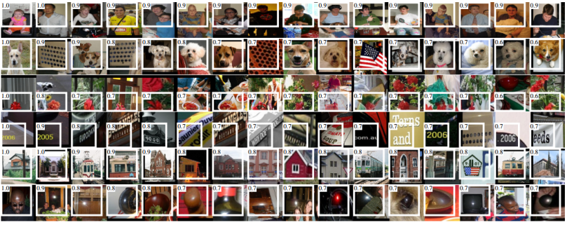
Figure 4: Top regions for six pool5 units. Receptive fields and activation values are drawn in white. Some units are aligned to concepts, such as people (row 1) or text (4). Other units capture texture and material properties, such as dot arrays (2) and specular reflections (6).

图4：六个pool5单元的激活最大的区域。感受野和激活值以白色绘制。某些单元与概念对齐，例如人（第1行）或文本（第4行）。其它单元捕获纹理和材料属性，如点阵列（第2行）和镜面反射（第6行）。）

3.2. Ablation studies

Performance layer-by-layer, without fine-tuning. To understand which layers are critical for detection performance, we analyzed results on the VOC 2007 dataset for each of the CNN’s last three layers. Layer pool5 was briefly described in Section 3.1. The final two layers are summarized below.

*逐层分析性能，没有微调。*为了了解哪些层对于检测性能至关重要，我们分析了CNN最后三层在VOC 2007数据集上的结果。上一节简要描述了pool5。最后两层总结如下【就是将骨干CNN不同层次提取得特征放到SVM中进行分类，看哪个层特征得效果好】。

Layer fc6 is fully connected to pool5 . To compute features, it multiplies a 4096×9216 weight matrix by the pool5 feature map (reshaped as a 9216-dimensional vector) and then adds a vector of biases. This intermediate vector is component-wise half-wave rectified (x ← max(0, x)).

层fc6完全连接到pool5。为了计算特征，它将pool5的特征图乘以一个4096×9216的权重矩阵（重构为9216维向量），然后加上一个偏置向量。最后应用ReLU线性纠正。

Layer fc7 is the final layer of the network. It is implemented by multiplying the features computed by fc6 by a 4096 × 4096 weight matrix, and similarly adding a vector of biases and applying half-wave rectification.

层fc7是网络的最后一层。这是通过将由fc6计算的特征乘以4096×4096权重矩阵来实现的，并且类似地加上了偏置向量并应用ReLU线性纠正。

We start by looking at results from the CNN without fine-tuning on PASCAL, i.e. all CNN parameters were pre-trained on ILSVRC 2012 only. Analyzing performance layer-by-layer (Table 2 rows 1-3) reveals that features from fc7 generalize worse than features from fc6. This means that 29%, or about 16.8 million, of the CNN’s parameters can be removed without degrading map. More surprising is that removing both fc7 and fc6 produces quite good results even though pool5 features are computed using only 6% of the CNN’s parameters. Much of the CNN’s representational power comes from its convolutional layers, rather than from the much larger densely connected layers. This finding suggests potential utility in computing a dense feature map, in the sense of HOG, of an arbitrary-sized image by using only the convolutional layers of the CNN. This representation would enable experimentation with sliding-window detectors, including DPM, on top of pool5 features.

我们首先来看看没有在PASCAL上进行微调的CNN的结果，即所有的CNN参数仅在ILSVRC 2012上进行了预训练。逐层分析性能（如上表，表2第1-3行）显示，fc7的特征总体上差于fc6的特征。这意味着可以删除CNN参数的29％或约1680万【4096X4096=16777216】，而不会降低map。更令人惊讶的是，即使使用仅6％的CNN参数来计算pool5特征，除去fc7和fc6也产生相当好的结果。 CNN的大部分表达能力来自其卷积层，而不是来自于更密集的全连接层。这一发现表明通过仅使用CNN的卷积层来计算任意大小图像的类似HOG意义上的密集特征图的潜在实用性。这种表示方式可以在pool5特征之上实现包括DPM在内的滑动窗口检测器。

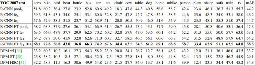
Table 2: Detection average precision (%) on VOC 2007 test. Rows 1-3 show R-CNN performance without fine-tuning. Rows 4-6 show results for the CNN pre-trained on ILSVRC 2012 and then fine-tuned (FT) on VOC 2007 trainval. Row 7 includes a simple bounding-box regression (BB) stage that reduces localization errors (Section C). Rows 8-10 present DPM methods as a strong baseline. The first uses only HOG, while the next two use different feature learning approaches to augment or replace HOG.

表2：VOC 2007测试集的检测平均精度（％）。第1-3行显示R-CNN没微调的性能。第4-6行显示CNN对ILSVRC 2012进行了预训练，然后对VOC 2007 trainval进行了微调（FT）的性能。第7行包括一个简单的边界框回归（BB）阶段，减少定位错误（C部分）。第8-10行将DPM方法作为强基线。第一次使用只有HOG，而接下来的两个使用不同的特征学习方法来增强或替换HOG。

Performance layer-by-layer, with fine-tuning. We now look at results from our CNN after having fine-tuned its parameters on VOC 2007 trainval. The improvement is striking (Table 2 rows 4-6): fine-tuning increases map by 8.0 percentage points to 54.2%. The boost from fine-tuning is much larger for fc6 and fc7 than for pool5 , which suggests that the pool5 features learned from ImageNet are general and that most of the improvement is gained from learning domain-specific non-linear classifiers on top of them.

*逐层分析性能，微调。*现在我们来看看在PASCAL上进行微调的CNN的结果。改善情况引人注目（表2第4-6行）：微调使map提高8.0个百分点至54.2％。对于fc6和fc7，微调的提升比对pool5大得多，这表明从ImageNet中学习的pool 5特性是一般性的，并且大多数改进是从学习域特定的非线性分类器获得的。

Comparison to recent feature learning methods. Relatively few feature learning methods have been tried on PASCAL VOC detection. We look at two recent approaches that build on deformable part models. For reference, we also include results for the standard HOG-based DPM [20].

*与近期特征学习方法的比较。*近期在PAS-CAL VOC检测中已经开始尝试了一些特征学习方法。我们来看两种最新的基于DPM模型的方法。作为参考，我们还包括基于标准HOG的DPM的结果20。

The first DPM feature learning method, DPM ST [28], augments HOG features with histograms of “sketch token” probabilities. Intuitively, a sketch token is a tight distribution of contours passing through the center of an image patch. Sketch token probabilities are computed at each pixel by a random forest that was trained to classify 35×35 pixel patches into one of 150 sketch tokens or background.

第一个DPM特征学习方法，DPM ST[28]，使用“草图表征”概率直方图增强了HOG特征。直观地，草图表征是通过图像片中心的轮廓的紧密分布。草图表征概率在每个像素处被随机森林计算，该森林经过训练，将35 x 35像素的图像片分类为150个草图表征或背景之一。

The second method, DPM HSC [31], replaces HOG with histograms of sparse codes (HSC). To compute an HSC, sparse code activations are solved for at each pixel using a learned dictionary of 100 7 × 7 pixel (grayscale) atoms. The resulting activations are rectified in three ways (full and both half-waves), spatially pooled, unit `2 normalized, and then power transformed (x ← sign(x)|x| α).

第二种方法，DPM HSC[31]，使用稀疏码直方图(HSC)替代HOG。为了计算HSC，使用100个7 x 7像素（灰度）元素的学习词典，在每个像素处求解稀疏代码激活。所得到的激活以三种方式整流（全部和两个半波），空间合并，单位L2归一化，和功率变换(x←sign(x)|x|α)(x←sign(x)|x|α)。

All R-CNN variants strongly outperform the three DPM baselines (Table 2 rows 8-10), including the two that use feature learning. Compared to the latest version of DPM, which uses only HOG features, our map is more than 20 percentage points higher: 54.2% vs. 33.7%—a 61% relative improvement. The combination of HOG and sketch tokens yields 2.5 map points over HOG alone, while HSC improves over HOG by 4 map points (when compared internally to their private DPM baselines—both use nonpublic implementations of DPM that underperform the open source version [20]). These methods achieve mAPs of 29.1% and 34.3%, respectively.

所有R-CNN的变体都优于三个DPM基线（表2第8-10行），包括两个使用特征学习的。与仅使用HOG特征的最新版本的DPM相比，我们的map提高了20个百分点以上：54.2％对比33.7％，相对改进61％。HOG和草图表征的组合与单独的HOG相比map提高2.5个点，而HSC在HOG上map提高了4个点（使用内部私有的DPM基线进行比较，两者都使用非公开实现的DPM，低于开源版本）。这些方法的map分别达到29.1％和34.3％。

3.3. Network architectures

Most results in this paper use the network architecture from Krizhevsky et al. [25]. However, we have found that the choice of architecture has a large effect on R-CNN detection performance. In Table 3 we show results on VOC 2007 test using the 16-layer deep network recently proposed by Simonyan and Zisserman [43]. This network was one of the top performers in the recent ILSVRC 2014 classification challenge. The network has a homogeneous structure consisting of 13 layers of 3 × 3 convolution kernels, with five max pooling layers interspersed, and topped with three fully-connected layers. We refer to this network as “O-Net” for OxfordNet and the baseline as “T-Net” for TorontoNet.

本文的大多数结果使用了Krizhevsky等人的网络架构。然而，我们发现架构的选择对R-CNN检测性能有很大的影响。在表3中，我们显示了使用Simonyan和Zisserman最近提出的16层深层网络的VOC 2007测试结果[43]。该网络是最近ILSVRC 2014分类挑战中表现最佳的网络之一。该网络具有由13层3×3卷积核组成的均匀结构，其中穿插有五个最大池化层，并且顶部有三个完全连接的层。我们将这个网络称为OxfordNet的“O-Net”，并将TorontoNet的基线称为“T-Net”。

To use O-Net in R-CNN, we downloaded the publicly available pre-trained network weights for the VGG ILSVRC 16 layers model from the Caffe Model Zoo.1 We then fine-tuned the network using the same protocol as we used for T-Net. The only difference was to use smaller minibatches (24 examples) as required in order to fit within GPU memory. The results in Table 3 show that RCNN with O-Net substantially outperforms R-CNN with TNet, increasing map from 58.5% to 66.0%. However there is a considerable drawback in terms of compute time, with the forward pass of O-Net taking roughly 7 times longer than T-Net.

要在R-CNN中使用O-Net，我们从Caffe模型库下载了预训练的VGG_ILSVRC_16_layers模型（https://github.com/BVLC/caffe/wiki/Model-Zoo）。然后我们使用与T-Net一样的方法对网络进行了微调。唯一的区别是根据需要使用较小的批量（24个），以适应GPU内存。表3中的结果显示，具有O-Net的R- CNN基本上优于T-网络的R-CNN，将map从58.5％提高到66.0％。然而，在计算时间方面存在相当大的缺陷，O-Net的前进速度比T-Net长约7倍。

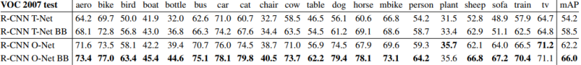
Table 3: Detection average precision (%) on VOC 2007 test for two different CNN architectures. The first two rows are results from Table 2 using Krizhevsky et al.’s architecture (T-Net). Rows three and four use the recently proposed 16-layer architecture from Simonyan and Zisserman (O-Net) [43].

表3：两种不同CNN架构的VOC 2007测试的检测平均精度（％）。前两行是表2中使用Krizhevsky等人的架构（T-Net）的结果。第三和第四行使用最近提出的Simonyan和Zisserman（O-Net）的16层架构[43]。

3.4. Detection error analysis

We applied the excellent detection analysis tool from Hoiem et al. [23] in order to reveal our method’s error modes, understand how fine-tuning changes them, and to see how our error types compare with DPM. A full summary of the analysis tool is beyond the scope of this paper and we encourage readers to consult [23] to understand some finer details (such as “normalized AP”). Since the analysis is best absorbed in the context of the associated plots, we present the discussion within the captions of Figure 5 and Figure 6.

为了揭示我们的方法的错误模式，我们应用了Hoiem等人的优秀检测分析工具23，以了解微调如何改变它们，并将我们的错误类型与DPM比较。分析工具的完整介绍超出了本文的范围，可以参考23了解更多的细节（如“标准化AP”）。千言万语不如一张图，我们在下图（图5和图6）中讨论。

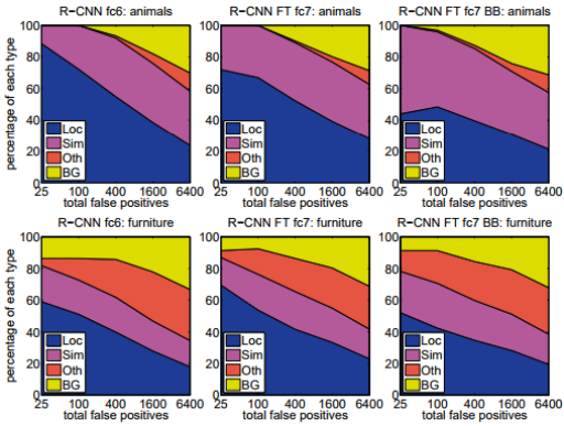
Figure 5: Distribution of top-ranked false positive (FP) types. Each plot shows the evolving distribution of FP types as more FPs are considered in order of decreasing score. Each FP is categorized into 1 of 4 types: Loc—poor localization (a detection with an IoU overlap with the correct class between 0.1 and 0.5, or a duplicate); Sim—confusion with a similar category; Oth—confusion with a dissimilar object category; BG—a FP that fired on background. Compared with DPM (see [23]), significantly more of our errors result from poor localization, rather than confusion with background or other object classes, indicating that the CNN features are much more discriminative than HOG. Loose localization likely results from our use of bottom-up region proposals and the positional invariance learned from pre-training the CNN for whole-image classification. Column three shows how our simple bounding-box regression method fixes many localization errors.

图5：最多的假阳性（FP）类型分布。每个图表显示FP类型的演变分布，按照FP数量降序排列。FP分为4种类型：Loc（定位精度差，检测框与真值的IoU在0.1到0.5之间或重复的检测）。Sim（与相似类别混淆）。Oth（与不相似的类别混淆）。BG（检测框标在了背景上）。与DPM（参见22）相比，我们的Loc显著增加，而不是Oth和BG，表明CNN特征比HOG更具区分度。Loc增加的原因可能是我们使用自下而上的区域提案可能产生松散的定位位置，以及CNN进行全图像分类的预训练模型所获得的位置不变性。第三列显示了我们的简单边界回归方法如何修复许多Loc【这个图不是很好看懂，是取每一条的面积来看？】。

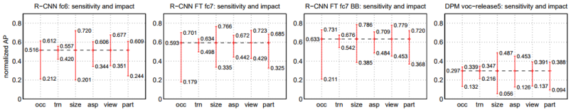
Figure 6: Sensitivity to object characteristics. Each plot shows the mean (over classes) normalized AP (see [23]) for the highest and lowest performing subsets within six different object characteristics (occlusion, truncation, bounding-box area, aspect ratio, viewpoint, part visibility).

对目标特点的敏感度。每个图显示六个不同目标特点（遮挡，截断，边界区域，纵横比，视角，局部可视性）内最高和最低性能的子集的平均值（跨类别）归一化AP（见22）。

We show plots for our method (R-CNN) with and without fine-tuning (FT) and bounding-box regression (BB) as well as for DPM voc-release5. Overall, fine-tuning does not reduce sensitivity (the difference between max and min), but does substantially improve both the highest and lowest performing subsets for nearly all characteristics. This indicates that fine-tuning does more than simply improve the lowest performing subsets for aspect ratio and bounding-box area, as one might conjecture based on how we warp network inputs. Instead, fine-tuning improves robustness for all characteristics including occlusion, truncation, viewpoint, and part visibility.

我们展示了我们的方法（R-CNN）有或没有微调（FT）和边界回归（BB）以及DPM voc-release5的图。总体而言，微调并不会降低敏感度（最大和最小值之间的差异），而且对于几乎所有的特点，都能极大地提高最高和最低性能的子集的性能。这表明微调不仅仅是简单地提高纵横比和边界区域的最低性能子集的性能（在分析之前，基于我们如何缩放网络输入而推测）。相反，微调可以改善所有特点的鲁棒性，包括遮挡，截断，视角和局部可视性。

3.5. Bounding-box regression

Based on the error analysis, we implemented a simple method to reduce localization errors. Inspired by the bounding-box regression employed in DPM [17], we train a linear regression model to predict a new detection window given the pool5 features for a selective search region proposal. Full details are given in Appendix C. Results in Table 1, Table 2, and Figure 5 show that this simple approach fixes a large number of mislocalized detections, boosting map by 3 to 4 points.

基于错误分析，我们实现了一种简单的方法来减少定位错误。受DPM中使用边界框回归的启发，我们训练一个线性回归模型使用在区域提案上提取的pool5特征来预测一个新的检测框。完整的细节在附录C中给出。表1，表2和图5中的结果表明，这种简单的方法解决了大量的定位错误，将map提高了3到4个点。

3.6. Qualitative results

Qualitative detection results on ILSVRC2013 are presented in Figure 8 and Figure 9 at the end of the paper. Each image was sampled randomly from the val2 set and all detections from all detectors with a precision greater than 0.5 are shown. Note that these are not curated and give a realistic impression of the detectors in action. More qualitative results are presented in Figure 10 and Figure 11, but these have been curated. We selected each image because it contained interesting, surprising, or amusing results. Here, also, all detections at precision greater than 0.5 are shown.

论文结尾处的图8和图9介绍了ILSVRC2013的定性检测结果。所有显示的图像都是从val2集中随机采样的，其精度大于0.5。请注意，这些都没有特意挑选，并给出了一个实际检测器的检测结果。更定性结果如图10和图11所示，这些都是专门挑选的。我们选择了每张图片，因为它包含有趣，令人惊讶或有趣的结果。这里，此外，还显示了精度大于0.5的所有检测。

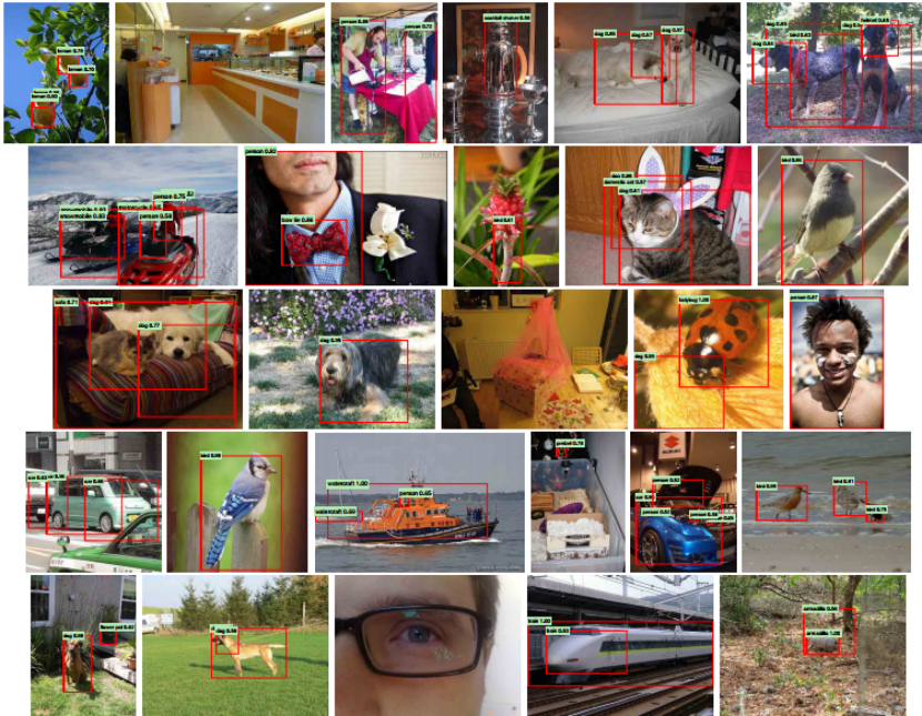
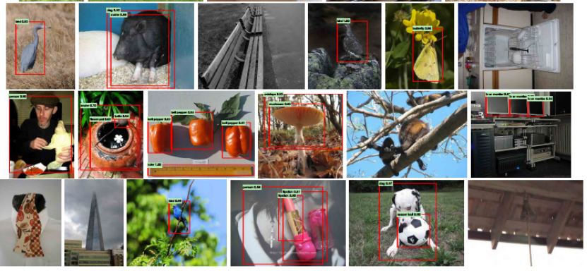
Figure 8: Example detections on the val2 set from the configuration that achieved 31.0% map on val2. Each image was sampled randomly (these are not curated). All detections at precision greater than 0.5 are shown. Each detection is labeled with the predicted class and the precision value of that detection from the detector’s precision-recall curve. Viewing digitally with zoom is recommended.

图8：在val2上达到31.0％map的配置的检测结果示例。每个图像都是随机抽样的（这些都没有刻意挑选）。显示精度大于0.5的所有检测，并标记了预测的类别和精度。可以放大以看清楚

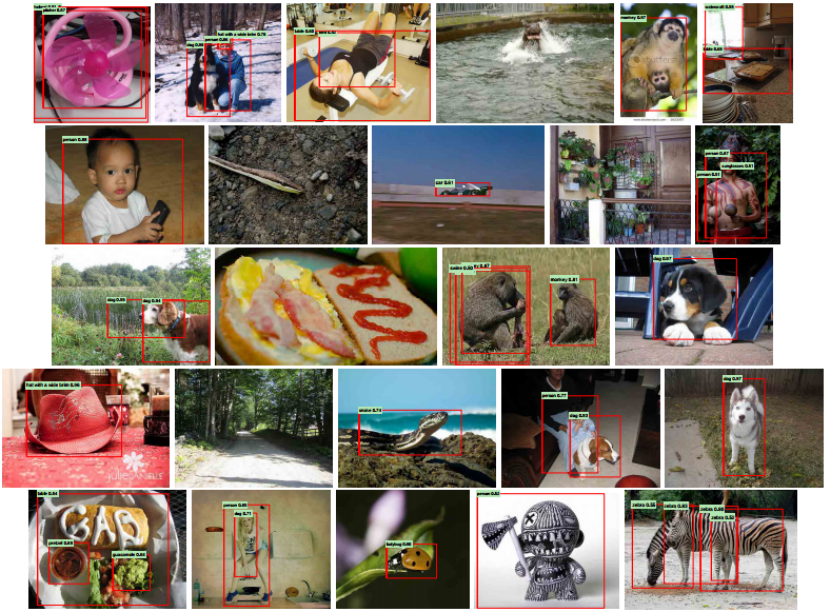
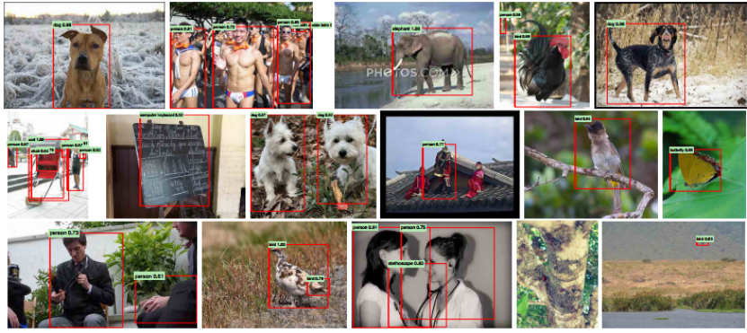
Figure 9: More randomly selected examples. See Figure 8 caption for details. Viewing digitally with zoom is recommended.

更多示例。详见图8说明。

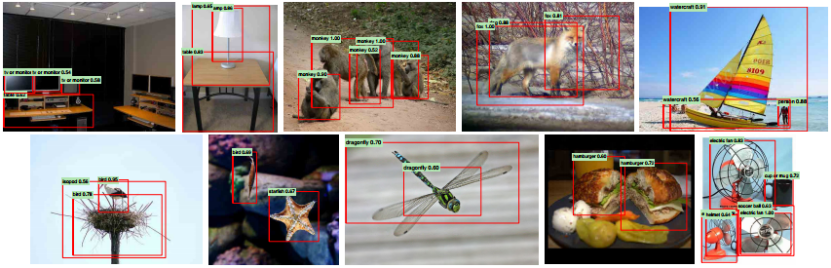
Figure 10: Curated examples. Each image was selected because we found it impressive, surprising, interesting, or amusing. Viewing digitally with zoom is recommended.

图10：挑选的示例。选择每张图片是因为我们发现它令人印象深刻，令人惊讶，有趣或有趣。建议使用缩放以数字方式查看

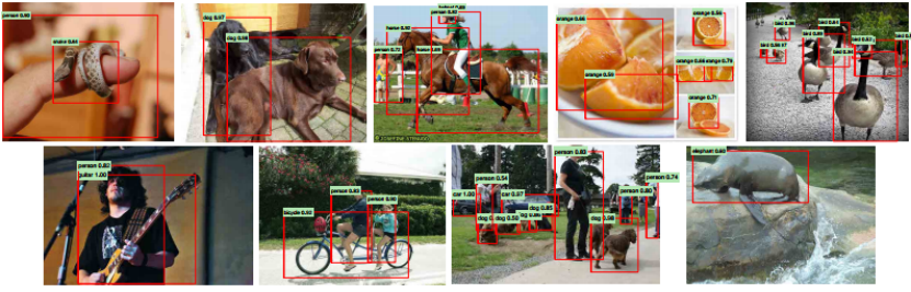
Figure 11: More curated examples. See Figure 10 caption for details. Viewing digitally with zoom is recommended.

图11：更多精选示例。有关详细信息，请参见图10标题。建议使用缩放以数字方式查看。

4. The ILSVRC2013 detection dataset

In Section 2 we presented results on the ILSVRC2013 detection dataset. This dataset is less homogeneous than PASCAL VOC, requiring choices about how to use it. Since these decisions are non-trivial, we cover them in this section.

在用R-CNN进行目标检测中，我们介绍了ILSVRC2013检测数据集的结果。该数据集与PASCAL VOC不太一致，需要选择如何使用它。由于这些选择不是显而易见的，我们将在这一节中介绍这些选择。

4.1. Dataset overview

The ILSVRC2013 detection dataset is split into three sets: train (395,918), val (20,121), and test (40,152), where the number of images in each set is in parentheses. The val and test splits are drawn from the same image distribution. These images are scene-like and similar in complexity (number of objects, amount of clutter, pose variability, etc.) to PASCAL VOC images. The val and test splits are exhaustively annotated, meaning that in each image all instances from all 200 classes are labeled with bounding boxes. The train set, in contrast, is drawn from the ILSVRC2013 classification image distribution. These images have more variable complexity with a skew towards images of a single centered object. Unlike val and test, the train images (due to their large number) are not exhaustively annotated. In any given train image, instances from the 200 classes may or may not be labeled. In addition to these image sets, each class has an extra set of negative images. Negative images are manually checked to validate that they do not contain any instances of their associated class. The negative image sets were not used in this work. More information on how ILSVRC was collected and annotated can be found in [11, 36].

ILSVRC2013检测数据集分为三组：训练(395,918)，验证(20,121)和测试(40,152)，其中每组的图像数目在括号中。验证和测试集是从相同的图像分布中划分的。这些图像与PASCAL VOC图像中的场景和复杂性（目标数量，杂波量，姿态变异性等）类似。验证和测试集是详尽标注的，这意味着在每个图像中，来自所有200个类的所有实例都被标注为边界框。相比之下，训练集来自ILSVRC2013分类图像。这些图像具有更多的可变复杂性，并且倾向于是单个位于图像中心的目标的图像。与验证和测试集不同，训练集（由于它们的数量很多）没有详尽标注。在任何给定的训练图像中，200个类别的实例可能被标注也可能不被标注。除了这些图像集，每个类都有一组额外的负样本。负样本经过人工检查以确认它们不包含任何相关类的实例。本文没有使用负样本。有关如何收集和标注ILSVRC的更多信息可以在[11,36]中找到。

The nature of these splits presents a number of choices for training R-CNN. The train images cannot be used for hard negative mining, because annotations are not exhaustive. Where should negative examples come from? Also, the train images have different statistics than val and test. Should the train images be used at all, and if so, to what extent? While we have not thoroughly evaluated a large number of choices, we present what seemed like the most obvious path based on previous experience.

这些数据集的分组的性质为训练R-CNN提供了许多选择。训练图像不能用于难负样本重训练，因为标注不是很好。负样本来自哪里？此外，训练图像具有不同于验证和训练集的分布。是否应该使用训练图像，如果是，在什么程度上？虽然我们还没有彻底评估大量的选择，但是我们根据以往的经验，提出了一个最明显的路径。

Our general strategy is to rely heavily on the val set and use some of the train images as an auxiliary source of positive examples. To use val for both training and validation, we split it into roughly equally sized “val1” and “val2” sets. Since some classes have very few examples in val (the smallest has only 31 and half have fewer than 110), it is important to produce an approximately class-balanced partition. To do this, a large number of candidate splits were generated and the one with the smallest maximum relative class imbalance was selected.2 Each candidate split was generated by clustering val images using their class counts as features, followed by a randomized local search that may improve the split balance. The particular split used here has a maximum relative imbalance of about 11% and a median relative imbalance of 4%. The val1/val2 split and code used to produce them will be publicly available to allow other researchers to compare their methods on the val splits used in this report.

我们的总体策略是严重依赖验证集，并使用一些训练图像作为一个辅助正样本来源。为了使用验证集进行训练和验证，我们将其分成大小大致相等的“val1”和“val2”集合。由于某些类在val中的数量非常少（最小的只有31个，连110个的一半都不到），所以产生一个近似类间均衡的划分是很重要的。为此，产生了大量的候选分割，并选择了最大相对类间不平衡的最小值（相对不平衡度被定义为|a-b|/(a+b)，其中a和b是两个集合各自的类计数）。每个候选分裂是通过使用其类计数作为特征聚类的验证集图像来生成的，然后是一个可以改善划分平衡度的随机局部搜索。这里使用的特定划分具有约11％的最大相对类间不平衡和4％的中值相对类间不平衡。val1/val2划分和用于生产它们的代码将被公开提供，以允许其他研究人员将他们的方法与在本文中使用的验证集划分方法进行比较。

4.2. Region proposals

We followed the same region proposal approach that was used for detection on PASCAL. Selective search [39] was run in “fast mode” on each image in val1, val2, and test (but not on images in train). One minor modification was required to deal with the fact that selective search is not scale invariant and so the number of regions produced depends on the image resolution. ILSVRC image sizes range from very small to a few that are several mega-pixels, and so we resized each image to a fixed width (500 pixels) before running selective search. On val, selective search resulted in an average of 2403 region proposals per image with a 91.6% recall of all ground-truth bounding boxes (at 0.5 IoU threshold). This recall is notably lower than in PASCAL, where it is approximately 98%, indicating significant room for improvement in the region proposal stage.

我们遵循用于PASCAL检测的区域提案方法。选择性搜索16在val1，val2中的每个图像上以“快速模式”运行，并进行测试（但不是在训练图像上）。需要一个小的修改来处理选择性搜索不是尺度不变的，所以需要产生的区域数量取决于图像分辨率。 ILSVRC的图像尺寸范围从非常小到少量几百万像素的图像，因此我们在运行选择性搜索之前，将每个图像的大小调整为固定的宽度（500像素）。在验证集上，选择性搜索在每个图像上平均有2403个区域提案，检测框真值（以0.5 IoU阈值）的召回率91.6％。这一召回率明显低于PASCAL的约98％，表明该区域提案阶段有明显的改善空间。

4.3. Training data

For training data, we formed a set of images and boxes that includes all selective search and ground-truth boxes from val1 together with up to N ground-truth boxes per class from train (if a class has fewer than N ground-truth boxes in train, then we take all of them). We’ll call this dataset of images and boxes val1+trainN . In an ablation study, we show map on val2 for N ∈ {0, 500, 1000} (Section 4.5).

对于训练数据，我们形成了一套图像和方框，其中包括val1的所有选择性搜索和检测框真值，以及训练集中每个类别最多N个检测框真值（如果一个类别的检测框真值数少于N个，那就有多少用多少）。我们将把这个数据集称为val1+trainN。在消融研究中，我们给出了N∈{0,500,1000}的val2上的map（见消融实验）。

Training data is required for three procedures in R-CNN: (1) CNN fine-tuning, (2) detector SVM training, and (3) bounding-box regressor training. CNN fine-tuning was run for 50k SGD iteration on val1+trainN using the exact same settings as were used for PASCAL. Fine-tuning on a single NVIDIA Tesla K20 took 13 hours using Caffe. For SVM training, all ground-truth boxes from val1+trainN were used as positive examples for their respective classes. Hard negative mining was performed on a randomly selected subset of 5000 images from val1. An initial experiment indicated that mining negatives from all of val1, versus a 5000 image subset (roughly half of it), resulted in only a 0.5 percentage point drop in map, while cutting SVM training time in half. No negative examples were taken from train because the annotations are not exhaustive. The extra sets of verified negative images were not used. The bounding-box regressors were trained on val1.

R-CNN中的三个阶段需要训练数据：（1）CNN微调，（2）检测器SVM训练（3）检测框回归训练。使用与用于PASCAL的完全相同的设置，在val1+trainN上进行50k次SGD迭代以微调CNN。使用Caffe在一块NVIDIA Tesla K20上微调花了13个小时。对于SVM训练，使用来自val1+trainN的所有检测框真值作为各自类别的正样本。对来自val1的5000张（大约一半）随机选择的图像的子集执行难负样本重训练。最初的实验表明，难负样本重训练仅使map下降了0.5个百分点，同时将SVM训练时间缩短了一半。没有从训练集中采样负样本，因为没有详尽标注。没有额外的经过确认的负样本。边界框回归器在val1训练。

4.4. Validation and evaluation

Before submitting results to the evaluation server, we validated data usage choices and the effect of fine-tuning and bounding-box regression on the val2 set using the training data described above. All system hyperparameters (e.g., SVM C hyperparameters, padding used in region warping, NMS thresholds, bounding-box regression hyperparameters) were fixed at the same values used for PASCAL. Undoubtedly some of these hyperparameter choices are slightly suboptimal for ILSVRC, however the goal of this work was to produce a preliminary R-CNN result on ILSVRC without extensive dataset tuning. After selecting the best choices on val2, we submitted exactly two result files to the ILSVRC2013 evaluation server. The first submission was without bounding-box regression and the second submission was with bounding-box regression. For these submissions, we expanded the SVM and boundingbox regressor training sets to use val+train1k and val, respectively. We used the CNN that was fine-tuned on val1+train1k to avoid re-running fine-tuning and feature computation.

在将结果提交给评估服务器之前，我们使用上述训练数据验证了数据使用选择、微调和检测框回归对val 2集的影响。所有系统超参数（例如，SVM C超参数，区域缩放中使用的边界填充，NMS阈值，检测框回归超参数）固定为与PASCAL相同的值。毫无疑问，这些超参数选择中的一些对ILSVRC来说稍微不太理想，但是这项工作的目标是在没有广泛数据集调优的情况下，在ILSVRC上产生初步的R-CNN结果。在选择val2上的最佳配置后，我们提交了两个结果文件到ILSVRC2013评估服务器。第一个没有检测框回归，第二个有检测框回归。对于这些提交，我们扩展了SVM和检测框回归训练集，分别使用val+train1k和val。我们在val1+train1k上微调CNN来避免重新运行微调和特征计算。

4.5. Ablation study

Table 4 shows an ablation study of the effects of different amounts of training data, fine-tuning, and boundingbox regression. A first observation is that map on val2 matches map on test very closely. This gives us confidence that map on val2 is a good indicator of test set performance. The first result, 20.9%, is what R-CNN achieves using a CNN pre-trained on the ILSVRC2012 classification dataset (no fine-tuning) and given access to the small amount of training data in val1 (recall that half of the classes in val1 have between 15 and 55 examples). Expanding the training set to val1+trainN improves performance to 24.1%, with essentially no difference between N = 500 and N = 1000. Fine-tuning the CNN using examples from just val1 gives a modest improvement to 26.5%, however there is likely significant overfitting due to the small number of positive training examples. Expanding the fine-tuning set to val1+train1k, which adds up to 1000 positive examples per class from the train set, helps significantly, boosting map to 29.7%. Bounding-box regression improves results to 31.0%, which is a smaller relative gain that what was observed in PASCAL.

如表（表4）所示：（ILSVRC2013上的数据使用选择、微调和边界回归消融研究。）第一个观察是，val2上的map与测试集上的map非常接近。这使我们有信心相信，val2上的map是测试集性能的良好指标。第一个结果是20.9％，是在ILSVRC2012分类数据集上预训练的CNN（无微调）并允许访问val1中少量训练数据的R-CNN实现（val1中一半的类别，每个类有15到55个样本）。将训练集扩展到val1+trainN将性能提高到24.1％，N = 500和N = 1000之间基本上没有差异。使用仅从val1的样本微调CNN可以稍微改善到26.5％，但是由于用于训练的正样本较少，可能会出现严重的过拟合。将用于微调的数据扩展到val1+train1k，相当于每个类增加了100个正样本用于训练，有助于将map显著提高至29.7％。检测框回归将结果提高到31.0％，这与PASCAL中所观察到的收益相比较小。

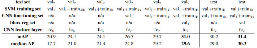
Table 4: ILSVRC2013 ablation study of data usage choices, fine-tuning, and bounding-box regression.

表4：ILSVRC2013上的数据使用选择、微调和边界回归消融研究。

4.6. Relationship to OverFeat

There is an interesting relationship between R-CNN and OverFeat: OverFeat can be seen (roughly) as a special case of R-CNN. If one were to replace selective search region proposals with a multi-scale pyramid of regular square regions and change the per-class bounding-box regressors to a single bounding-box regressor, then the systems would be very similar (modulo some potentially significant differences in how they are trained: CNN detection fine-tuning, using SVMs, etc.). It is worth noting that OverFeat has a significant speed advantage over R-CNN: it is about 9x faster, based on a figure of 2 seconds per image quoted from [34]. This speed comes from the fact that OverFeat’s sliding windows (i.e., region proposals) are not warped at the image level and therefore computation can be easily shared between overlapping windows. Sharing is implemented by running the entire network in a convolutional fashion over arbitrary-sized inputs. Speeding up R-CNN should be possible in a variety of ways and remains as future work.

R-CNN和OverFeat之间有一个有趣的关系：OverFeat可以看作（大致上）是R-CNN的一个特例。如果用一个多尺度的正方形区域的金字塔取代选择性搜索区域提案，并将每个类别的检测框回归器改变为一个单一的检测框回归函数，则两个系统将是非常相似的（训练上有一些潜在的显著差异：CNN微调、使用SVM等）。值得注意的是，OverFeat比R-CNN具有显着的速度优势：根据18引用的图中显示每张图像2秒，速度约为RCNN的9倍。这种速度来自于OverFeat的滑动窗口（即区域提案）在图像级别没有缩放的事实，因此可以在重叠窗口之间轻松共享计算。通过在任意大小的输入上以卷积方式运行整个网络来实现共享。加快R-CNN的速度应该有很多可行的办法，未来的工作中将会考虑。

5. Semantic segmentation

Region classification is a standard technique for semantic segmentation, allowing us to easily apply R-CNN to the PASCAL VOC segmentation challenge. To facilitate a direct comparison with the current leading semantic segmentation system (called O2P for “second-order pooling”) [4], we work within their open source framework. O2P uses CPMC to generate 150 region proposals per image and then predicts the quality of each region, for each class, using support vector regression (SVR). The high performance of their approach is due to the quality of the CPMC regions and the powerful second-order pooling of multiple feature types (enriched variants of SIFT and LBP). We also note that Farabet et al. [16] recently demonstrated good results on several dense scene labeling datasets (not including PASCAL) using a CNN as a multi-scale per-pixel classifier.

区域分类是语义分割的基础，这使我们可以轻松地将R-CNN应用于PASCAL VOC分割挑战。为了便于与当前领先的语义分割系统（称为“二阶池化”的O2P）的直接比较，我们在其开源框架内修改。O2P使用CPMC为每个图像生成150个区域提案，然后使用支持向量回归(SVR)来预测对于每个类别的每个区域的质量。他们的方法的高性能是由于CPMC区域的高质量和强大的多种特征类型（SIFT和LBP的丰富变体）的二阶池化。我们还注意到，Farabet等最近使用CNN作为多尺度像素级分类器在几个密集场景标记数据集（不包括PAS-CAL）上取得了良好的结果。

We follow [2, 4] and extend the PASCAL segmentation training set to include the extra annotations made available by Hariharan et al. [22]. Design decisions and hyperparameters were cross-validated on the VOC 2011 validation set. Final test results were evaluated only once.

我们遵循并扩展PASCAL分割训练集，以包含Hariharan等提供的额外注释。在VOC 2011验证集上，交叉验证我们的设计决策和超参数。最终测试结果仅提交一次。

CNN features for segmentation. We evaluate three strategies for computing features on CPMC regions, all of which begin by warping the rectangular window around the region to 227 × 227. The first strategy (full) ignores the region’s shape and computes CNN features directly on the warped window, exactly as we did for detection. However, these features ignore the non-rectangular shape of the region. Two regions might have very similar bounding boxes while having very little overlap. Therefore, the second strategy (fg) computes CNN features only on a region’s foreground mask. We replace the background with the mean input so that background regions are zero after mean subtraction. The third strategy (full+fg) simply concatenates the full and fg features; our experiments validate their complementarity.

*用于分割的CNN特征。*我们评估了在CPMC区域上计算特征的三个策略，所有这些策略都是将区域缩放为227 x 227。第一个策略（full）忽略了该区域的形状，并直接在缩放后的区域上计算CNN特征，就像我们缩放区域提案那样。然而，这些特征忽略了区域的非矩形形状。两个区域可能具有非常相似的边界框，同时具有非常小的重叠。因此，第二个策略（fg）仅在区域的前景掩码上计算CNN特征。我们用图像均值替换背景，使得背景区域在减去图像均值后为零。第三个策略（full + fg）简单地连接full和fg特征。我们的实验验证了它们的互补性。

Results on VOC 2011. Table 5 shows a summary of our results on the VOC 2011 validation set compared with O2P. (See Appendix E for complete per-category results.) Within each feature computation strategy, layer fc6 always outperforms fc7 and the following discussion refers to the fc6 features. The fg strategy slightly outperforms full, indicating that the masked region shape provides a stronger signal, matching our intuition. However, full+fg achieves an average accuracy of 47.9%, our best result by a margin of 4.2% (also modestly outperforming O2P), indicating that the context provided by the full features is highly informative even given the fg features. Notably, training the 20 SVRs on our full+fg features takes an hour on a single core, compared to 10+ hours for training on O2P features.

关于VOC 2011的结果。表5显示了我们在VOC 2011验证集上与O2P相比的结果，每个类别的完整结果参见附录E。在每种特征计算策略中，fc6总是超过fc7，以下讨论是指fc6的特征。fg策略稍微优于full，表明掩码区域的形状提供了更强的信号，与我们的直觉相匹配。然而，full + fg的平均准确度达到47.9％，比我们的fg最佳结果高4.2％（也略胜于O2P），表明full特征提供大量的信息，即使给定fg特征。值得注意的是，在full + fg特征上使用一个CPU核心训练20个SVR需要花费一个小时，相比之下，在O2P特征上训练需要10个多小时。

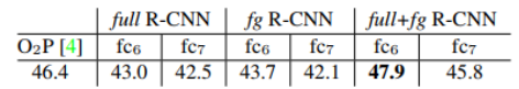
Table 5: Segmentation mean accuracy (%) on VOC 2011 validation. Column 1 presents O2P; 2-7 use our CNN pre-trained on ILSVRC 2012.

表5：VOC 2011验证的分段平均准确度（％）。第1列呈现O2P; 2-7使用我们的CNN预训练

ILSVRC 2012。

In Table 6 we present results on the VOC 2011 test set, comparing our best-performing method, fc6 (full+fg), against two strong baselines. Our method achieves the highest segmentation accuracy for 11 out of 21 categories, and the highest overall segmentation accuracy of 47.9%, averaged across categories (but likely ties with the O2P result under any reasonable margin of error). Still better performance could likely be achieved by fine-tuning.

在表6我们提供了VOC 2011测试集的结果，将我们的最佳表现方法fc6(full + fg)与两个强大的基线进行了比较。我们的方法在21个类别中的11个中达到了最高的分割精度，最高的分割精度为47.9％，跨类别平均（但可能与任何合理的误差范围内的O2P结果有关）。微调可能会实现更好的性能。

Table 6: Segmentation accuracy (%) on VOC 2011 test. We compare against two strong baselines: the “Regions and Parts” (R&P) method of [2] and the second-order pooling (O2P) method of [4]. Without any fine-tuning, our CNN achieves top segmentation performance, outperforming R&P and roughly matching O2P.

表6：VOC 2011测试的分段准确度（％）。我们比较两个强大的基线：“区域和部分”（R＆P）[2]的方法和[4]的二阶合并（O2P）方法。没有任何微调，我们的CNN实现了最高的细分性能，优于R＆P并大致匹配O2P。

6. Conclusion

In recent years, object detection performance had stagnated. The best performing systems were complex ensembles combining multiple low-level image features with high-level context from object detectors and scene classifiers. This paper presents a simple and scalable object detection algorithm that gives a 30% relative improvement over the best previous results on PASCAL VOC 2012.

近年来，物体检测性能停滞不前。性能最好的系统是复杂的组合，将多个低级图像特征与来自物体检测器和场景分类器的高级语境相结合。本文提出了一种简单且可扩展的对象检测算法，相对于PASCAL VOC 2012上的前最佳结果，相对改进了30％。

We achieved this performance through two insights. The first is to apply high-capacity convolutional neural networks to bottom-up region proposals in order to localize and segment objects. The second is a paradigm for training large CNNs when labeled training data is scarce. We show that it is highly effective to pre-train the network— with supervision—for a auxiliary task with abundant data (image classification) and then to fine-tune the network for the target task where data is scarce (detection). We conjecture that the “supervised pre-training/domain-specific finetuning” paradigm will be highly effective for a variety of data-scarce vision problems.

我们通过两个关键的改进实现了这一效果。第一个是将大容量卷积神经网络应用于自下而上的区域提案，以便定位和分割对象。第二个是在有标记的训练数据很少的情况下训练大型CNN的方法。我们发现，通过使用大量的图像分类数据对辅助任务进行有监督的预训练，然后对数据稀缺的目标检测任务进行微调，是非常有效的。我们相信，“监督的预训练/领域特定的微调”的方法对于各种数据缺乏的视觉问题都将是非常有效的。

We conclude by noting that it is significant that we achieved these results by using a combination of classical tools from computer vision and deep learning (bottom-up region proposals and convolutional neural networks). Rather than opposing lines of scientific inquiry, the two are natural and inevitable partners.

我们通过使用计算机视觉中的经典工具与深度学习（自下而上的区域提案和卷积神经网络）的组合达到了很好的效果。而不是仅仅依靠纯粹的科学探究。

Acknowledgments. This research was supported in part by DARPA Mind’s Eye and MSEE programs, by NSF awards IIS-0905647, IIS-1134072, and IIS-1212798, MURI N000014-10-1-0933, and by support from Toyota. The GPUs used in this research were generously donated by the NVIDIA Corporation.

*致谢：*该研究部分由DARPA Mind的Eye与MSEE项目支持，NSF授予了IIS-0905647，IIS-1134072和IIS-1212798，以及丰田支持的MURI N000014-10-1-0933。本研究中使用的GPU由NVIDIA公司慷慨捐赠。

Appendix A.

A. Object proposal transformations

The convolutional neural network used in this work requires a fixed-size input of 227 × 227 pixels. For detection, we consider object proposals that are arbitrary image rectangles. We evaluated two approaches for transforming object proposals into valid CNN inputs.

本文中使用的卷积神经网络需要227×227像素的固定大小输入。为了检测，我们认为目标提案是任意矩形的图像。我们评估了将目标提案转换为有效的CNN输入的两种方法。

The first method (“tightest square with context”) encloses each object proposal inside the tightest square and then scales (isotropically) the image contained in that square to the CNN input size. Figure 7 column (B) shows this transformation. A variant on this method (“tightest square without context”) excludes the image content that surrounds the original object proposal. Figure 7 column (C) shows this transformation. The second method (“warp”) anisotropically scales each object proposal to the CNN input size. Figure 7 column (D) shows the warp transformation.

第一个方法将目标提案扩充为正方形并缩放到所需大小，如图7(B)所示。这种方法还有一种变体，仅扩充为方框，扩充部分不填充图像内容，如图7(C)所示。第二种方法是将目标提案不保留横纵比的情况下缩放到所需大小，如图7(D)所示。

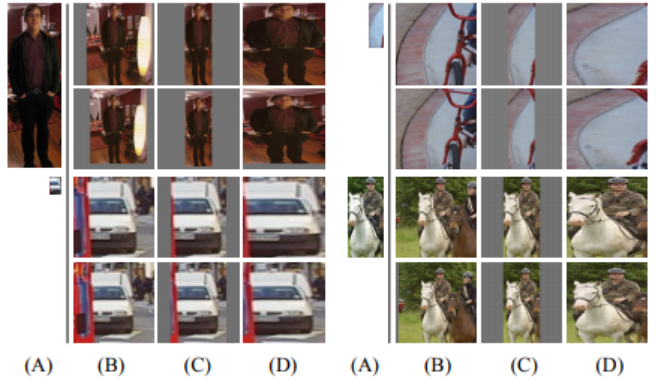
Figure 7: Different object proposal transformations. (A) the original object proposal at its actual scale relative to the transformed CNN inputs; (B) tightest square with context; (C) tightest square without context; (D) warp. Within each column and example proposal, the top row corresponds to p = 0 pixels of context padding while the bottom row has p = 16 pixels of context padding.

图7：不同的对象提议转换。（一）原始对象提案的实际规模相对于转换的CNN输入; （B）具有背景的最严格的正方形; （C）最紧张没有背景的广场; （D）翘曲。在每列内和示例提议，顶行对应于上下文的p = 0像素填充，而底行有p = 16像素的上下文填充。

For each of these transformations, we also consider including additional image context around the original object proposal. The amount of context padding (p) is defined as a border size around the original object proposal in the transformed input coordinate frame. Figure 7 shows p = 0 pixels in the top row of each example and p = 16 pixels in the bottom row. In all methods, if the source rectangle extends beyond the image, the missing data is replaced with the image mean (which is then subtracted before inputing the image into the CNN). A pilot set of experiments showed that warping with context padding (p = 16 pixels) outperformed the alternatives by a large margin (3-5 map points). Obviously more alternatives are possible, including using replication instead of mean padding. Exhaustive evaluation of these alternatives is left as future work.

对于这些转换中的每一个，我们还考虑在原始目标提案四周包括附加图像内容。内容填充的量(pp)被定义为在缩放后图像中，原始目标提案周围的边界大小。图7显示了每个示例的顶行中p=0像素，底行中p=16像素。在所有方法中，如果矩形框超出图像边缘，超出的部分将被填充为图像均值（然后在将图像输入到CNN之前减去）。一组实验表明，采用上下文填充（ p=16像素）的缩放可以明显提高map（提高3-5个点）。显然还有更多其它可行的方案，包括使用复制而不是平均填充。对这些方案的详尽评估将作为未来的工作。

B. Positive vs. negative examples and softmax

Two design choices warrant further discussion. The first is: Why are positive and negative examples defined differently for fine-tuning the CNN versus training the object detection SVMs? To review the definitions briefly, for finetuning we map each object proposal to the ground-truth instance with which it has maximum IoU overlap (if any) and label it as a positive for the matched ground-truth class if the IoU is at least 0.5. All other proposals are labeled “background” (i.e., negative examples for all classes). For training SVMs, in contrast, we take only the ground-truth boxes as positive examples for their respective classes and label proposals with less than 0.3 IoU overlap with all instances of a class as a negative for that class. Proposals that fall into the grey zone (more than 0.3 IoU overlap, but are not ground truth) are ignored.

有两个设计选择值得进一步讨论。第一个是：为什么在微调CNN和训练目标检测SVM时定义的正负样本不同？首先简要回顾下正负样本的定义，对于微调，我们将每个目标提案映射到它具有最大IoU重叠（如果有的话）的检测框真值上，如果其IoU至少为0.5，并将其标记为对应类别的正样本。剩下的提案都标记为“背景”（即所有类的负样本）。对于训练SVM，相比之下，我们只采用检测框真值作为各自类别的正样本。与某一类别所有的正样本的IoU都小于0.3的目标提案将被标记为该类别的负样本。其它（IoU超过0.3，但不是检测框真值）的提案被忽略。

Historically speaking, we arrived at these definitions because we started by training SVMs on features computed by the ImageNet pre-trained CNN, and so fine-tuning was not a consideration at that point in time. In that setup, we found that our particular label definition for training SVMs was optimal within the set of options we evaluated (which included the setting we now use for fine-tuning). When we started using fine-tuning, we initially used the same positive and negative example definition as we were using for SVM training. However, we found that results were much worse than those obtained using our current definition of positives and negatives.

从时序上讲，我们得出这些定义是因为我们一开始通过由ImageNet预先训练的CNN计算出的特征训练SVM，因此微调在这个时间点不是一个需要考虑因素。在这种情况下，我们发现，在我们评估的一组设置（包括我们现在用于微调的设置）中，我们当前使用的训练SVM的设置是最佳的。当我们开始使用微调时，我们最初使用与我们用于SVM训练的正负样本的定义相同的定义。然而，我们发现结果比使用我们当前定义的正负样本获得的结果差得多。

Our hypothesis is that this difference in how positives and negatives are defined is not fundamentally important and arises from the fact that fine-tuning data is limited. Our current scheme introduces many “jittered” examples (those proposals with overlap between 0.5 and 1, but not ground truth), which expands the number of positive examples by approximately 30x. We conjecture that this large set is needed when fine-tuning the entire network to avoid overfitting. However, we also note that using these jittered examples is likely suboptimal because the network is not being fine-tuned for precise localization.

我们的假设是，如何定义正负样本的差异对训练结果影响不大，结果的差异主要是由微调数据有限这一事实引起的。我们目前的方案引入了许多“抖动”的样本（这些提案与检测框真值的重叠在0.5和1之间，但并不是检测框真值），这将正样本的数量增加了大约30倍。我们推测，需要使用如此大量的样本以避免在微调网络时的过拟合。然而，我们还注意到，使用这些抖动的例子可能不是最佳的，因为网络没有被微调以进行精确的定位。

This leads to the second issue: Why, after fine-tuning, train SVMs at all? It would be cleaner to simply apply the last layer of the fine-tuned network, which is a 21-way softmax regression classifier, as the object detector. We tried this and found that performance on VOC 2007 dropped from 54.2% to 50.9% map. This performance drop likely arises from a combination of several factors including that the definition of positive examples used in fine-tuning does not emphasize precise localization and the softmax classifier was trained on randomly sampled negative examples rather than on the subset of “hard negatives” used for SVM training.

这导致了第二个问题：为什么微调之后，训练SVM呢？简单地将最后一层微调网络（21路Softmax回归分类器）作为对象检测器将变得更加简洁。我们尝试了这一点，发现VOC 2007的表现从54.2％下降到了50.9％的map。这种性能下降可能来自几个因素的组合，包括微调中使用的正样本的定义不强调精确定位，并且softmax分类器是在随机抽样的负样本上训练的，而不是用于训练SVM的“更严格的负样本”子集。

This result shows that it’s possible to obtain close to the same level of performance without training SVMs after fine-tuning. We conjecture that with some additional tweaks to fine-tuning the remaining performance gap may be closed. If true, this would simplify and speed up R-CNN training with no loss in detection performance.

这个结果表明，微调之后可以获得接近SVM水平的性能，而无需训练SVM。我们推测，通过一些额外的调整来微调以达到更接近的水平。如果是这样，这样可以简化和加速R-CNN训练，而不会在检测性能方面有任何损失。

C. Bounding-box regression

We use a simple bounding-box regression stage to improve localization performance. After scoring each selective search proposal with a class-specific detection SVM, we predict a new bounding box for the detection using a class-specific bounding-box regressor. This is similar in spirit to the bounding-box regression used in deformable part models [17]. The primary difference between the two approaches is that here we regress from features computed by the CNN, rather than from geometric features computed on the inferred DPM part locations.

我们使用一个简单的检测框回归来提高定位性能。在使用类特定检测SVM对每个选择性搜索提案进行评分之后，我们使用类别特定的边界回归器预测新的检测框。这与在可变部件模型中使用的检测框回归相似19。这两种方法之间的主要区别在于，我们使用CNN计算的特征回归，而不是使用在推测的DPM部件位置上计算的几何特征。

The input to our training algorithm is a set of N training pairs {(P i , Gi )}i=1,...,N , where P i = (P ix , Piy , Piw, Pih ) specifies the pixel coordinates of the center of proposal P i ’s bounding box together with P i ’s width and height in pixels. Hence forth, we drop the superscript i unless it is needed. Each ground-truth bounding box G is specified in the same way: G = (Gx, Gy, Gw, Gh). Our goal is to learn a transformation that maps a proposed box P to a ground-truth box G.

我们的训练算法的输入是一组N个训练对(Pi,Gi)i=1,…,N，其中Pi=(Pix,Piy,Piw,Pih)指定提案Pi的边界框中心的像素坐标以及宽度和高度（以像素为单位）。注意，除非需要，下文中我们不再写出上标i。每个检测框真值G以相同的方式指定：G=(Gx,Gy,Gw,Gh)。我们的目标是学习将提案框PP映射到检测框真值G的转换。

We parameterize the transformation in terms of four functions dx(P), dy(P), dw(P), and dh(P). The first two specify a scale-invariant translation of the center of P’s bounding box, while the second two specify log-space translations of the width and height of P’s bounding box. After learning these functions, we can transform an input proposal P into a predicted ground-truth box Gˆ by applying the transformation

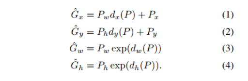
我们使用四个函数dx(P)，d(yP)，d(Pw)和dh(P)参数化这个转换。前两个指定P的边界框的中心的比例不变的平移，后两个指定PP的边界框的宽度和高度的对数空间转换。在学习了这些函数后，我们可以通过应用转换将输入提案P转换成预测的检测框真值G^。

每个函数d⋆(P)d⋆(P)（⋆⋆表示x,y,w,h中的一个）都建模为提案P的pool5特征（记为ϕ5(P)，对图像数据的依赖隐含的假定）的线性函数。即d⋆(P)=wT⋆ϕ5(P)，其中w⋆表示模型和训练参数的一个向量，通过优化正则化最小二乘法的目标（脊回归）来学习w⋆。

We found two subtle issues while implementing bounding-box regression. The ﬁrst is that regularization is important: we set λ = 1000 based on a validation set. The second issue is that care must be taken when selecting which training pairs (P,G) to use. Intuitively, if P is far from all ground-truth boxes, then the task of transforming P to a ground-truth box G does not make sense. Using examples like P would lead to a hopeless learning problem. Therefore, we only learn from a proposal P if it is nearby at least one ground-truth box. We implement “nearness” by assigning P to the ground-truth box G with which it has maximum IoU overlap (in case it overlaps more than one) if and only if the overlap is greater than a threshold (which we set to 0.6 using a validation set). All unassigned proposals are discarded. We do this once for each object class in order to learn a set of class-speciﬁc bounding-box regressors.

我们在实现边界框回归的时候发现了两个微妙的问题。第一个就是正则化是非常重要的：基于验证集，我们设置λ=1000。第二个问题是，在选择使用哪个训练对（P；G）时必须小心。直观地，如果远离所有的真实框，那么将P转换到真实框G的任务就没有意义。使用像P这样的例子将会导致一个无望的学习问题。因此，我们只从这样的候选P中进行学习，其至少与一个真实框离的比较近。我们通过将P分配给真实框G，当且仅当重叠大于阈值（我们使用一个验证集设置成0.6）时，它与其具有最大的IoU重叠（以防重叠超过一个）。所有未分配的候选区域都被丢弃。对于每一个对象类我们只做一次，以便学习一组特定类边界框的回归器。

At test time, we score each proposal and predict its new detection window only once. In principle, we could iterate this procedure (i.e., re-score the newly predicted bounding box, and then predict a new bounding box from it, and so on). However, we found that iterating does not improve results.

在测试的时候，我们为每一个候选框打分，并且预测一次它的新检测窗口。原则上来说，我们可以迭代这个过程（即，为新得到的预测框重新打分，然后从它再预测一个新的边界框，以此类推）。然而，我们发现迭代没有改善结果。

D. Additional feature visualizations

Figure 12 shows additional visualizations for 20 pool5 units. For each unit, we show the 24 region proposals that maximally activate that unit out of the full set of approximately 10 million regions in all of VOC 2007 test. We label each unit by its (y, x, channel) position in the 6 × 6 × 256 dimensional pool5 feature map. Within each channel, the CNN computes exactly the same function of the input region, with the (y, x) position changing only the receptive ﬁeld.

图12为20个pool5单元展示了附加的可视化。对于每一个单元来说，我们展示了可以最大激活VOC 2007 测试集的全部的大约1000万个区域中的24个候选区域。我们在6∗6∗256维的pool5特征图上为每个单元都标记了它的（y,x,channel）位置。在每个通道内，CNN计算输入区域的完全相同的函数。

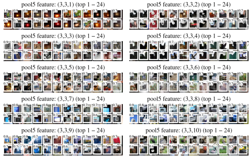
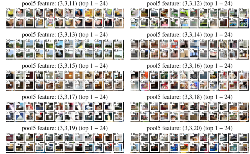
Figure 12: We show the 24 region proposals, out of the approximately 10 million regions in VOC 2007 test, that most strongly activate each of 20 units. Each montage is labeled by the unit’s (y, x, channel) position in the 6×6×256 dimensional pool5 feature map. Each image region is drawn with an overlay of the unit’s receptive ﬁeld in white. The activation value (which we normalize by dividing by the max activation value over all units in a channel) is shown in the receptive ﬁeld’s upper-left corner. Best viewed digitally with zoom.

图12：我们展示了在VOC2007测试中大约1000万个候选区域中的24个候选区域，其最强烈地激活20个单元中的每一个。每个剪辑都用6∗6∗256维的5pool5特征图的单元（y, x, channel）的位置标记。每一个图像区域都用白色的单元的感受野的覆盖图绘制。激活值（我们通过除以通道中所有单元的最大激活值来进行归一化）显示在接受域的左上角。建议放大来看

E. Per-category segmentation results

In Table 7 we show the per-category segmentation accuracy on VOC 2011 val for each of our six segmentation methods in addition to the O2P method [4]. These results show which methods are strongest across each of the 20 PASCAL classes, plus the background class.

在表7中，我们展示了我们6个分割方法中的每一个（除了O2PO2P方法）在VOC 2011val集上的每类分割准确度。这些结果展示了对于20个PASCAL类别加上背景类，哪一个方法是最强的。

![img](file:////tmp/wps-linxu/ksohtml/wpsKfy8ga.jpg)

Table7: Per-category segmentation accuracy (%) on the VOC 2011 validation set

F. Analysis of cross-dataset redundancy

One concern when training on an auxiliary dataset is that there might be redundancy between it and the test set. Even though the tasks of object detection and whole-image classiﬁcation are substantially different, making such cross-set redundancy much less worrisome, we still conducted thorough investigation that quantiﬁes the extent to which PASCAL test images are contained within the ILSVRC 2012 training and validation sets. Our ﬁndings may be useful to researchers who are interested in using ILSVRC 2012 as training data for the PASCAL image classiﬁcation task. We performed two checks for duplicate (and near duplicate) images. The ﬁrst test is based on exact matches of ﬂickr image IDs, which are included in the VOC 2007 test annotations (these IDs are intentionally kept secret for subsequent PASCAL test sets). All PASCAL images, and about half of ILSVRC, were collected from ﬂickr.com. This check turned up 31 matches out of 4952 (0.63%).

当在辅助数据集上进行训练时，一个问题是它与测试集之间可能存在冗余。即使对象检测和整个图像分类的任务有很大的不同，为了使这种交叉冗余不那么令人担忧，我们仍然进行了彻底的调查，量化了PASCAL测试图像包含在ILSVRC2012训练和验证集的程度。我们发现可能对那些有兴趣使用ILSVRC2012作为PASCAL图像分类任务的训练数据的研究人员有用。我们对重复（和近重复）图像执行了再次检查。第一个测试是基于flicker图像ID的精确匹配，这些ID包括在VOC 2007测试注释中（这些ID有意的为后续的PASCAL测试集保密）。所有的PASCAL图像，和约一半的ILSVRC图像，从flickr.com收集。这个检查证明了在4952有31个匹配（0.63%）。

The second check uses GIST [30] descriptor matching, which was shown in [13] to have excellent performance at near-duplicate image detection in large (> 1million) image collections. Following [13], we computed GIST descriptors on warped 32×32 pixel versions of all ILSVRC 2012 trainval and PASCAL 2007 test images. Euclidean distance nearest-neighbor matching of GIST descriptors revealed 38 near-duplicate images (including all 31 found by ﬂickr ID matching). The matches tend to vary slightly in JPEG compression level and resolution, and to a lesser extent cropping. These ﬁndings show that the overlap is small, less than 1%. For VOC 2012, because ﬂickr IDs are not available, we used the GIST matching method only. Based on GIST matches, 1.5% of VOC 2012 test images are in ILSVRC 2012 trainval. The slightly higher rate for VOC 2012 is likely due to the fact that the two datasets were collected closer together in time than VOC 2007 and ILSVRC 2012 were.

第二个检测使用了GIST描述符匹配，在[13]中显示在大（>100万）图像集合中的近似图像检测中具有优异的性能。在[13]之后，我们计算了所有的ILSVRC2012trainval和PASCAL 2007测试图像的扭曲32*32像素版本上的GIST描述符。GIST描述符的欧氏距离最近邻匹配揭示了38个近似重复图像（包括通过flickrID匹配找到的31个）。匹配在JPEG压缩级别和分辨率略有变化，并且趋向较小程度的裁剪。这些发现表明重叠是小的，小于1%。对于VOC 2012来说，因为flickrID是不可用的，我们只使用了GIST匹配方法。基于GIST匹配，VOC 2012测试图像的1.5%是在ILSVRC 2012trainval中的。对于VOC 2012略高的比率可能是由于这两个数据集在时间上收集的比VOC 2007和ILSVRC 2012更接近。

G. Document change log

This document tracks the progress of R-CNN. To help readers understand how it has changed over time, here’s a brief change log describing the revisions.

v1 Initial version.

v2 CVPR 2014 camera-ready revision. Includes substantial improvements in detection performance brought about by(1) starting ﬁne-tuning from a higher learning rate(0.001 instead of 0.0001), (2) using context padding when preparing CNN inputs, and (3) bounding-box regression to ﬁx localization errors.

v3 Results on the ILSVRC2013 detection dataset and comparison with OverFeat were integrated into several sections (primarily Section 2 and Section 4).

v4 The softmax vs. SVM results in Appendix B contained an error, which has been ﬁxed. We thank Sergio Guadarrama for helping to identify this issue.

v5 Added results using the new 16-layer network architecture from Simonyan and Zisserman [43] to Section 3.3 and Table 3.

本文跟踪的R-CNN的进度。为了帮助读者它是怎样随着时间改变的，这里是一个简明的更改日志描述了这些修定。
*V1* 最初的版本
*V2* CVPR相机就绪版本。包括在检测性能上的大量改进，由以下带来的：（1）以更高的学习率开始微调（0.001而不是0.0001），（2）当准备CNN时使用上下文填充，（3）边界框回归用于修复定位误差。
*V3* 在ILSVRC 2013检测数据集上的结果，并且与OverFeat的比较被集成到几个章节内（主要在第2和第4节）。
*V4* 在附录B上的softmax对SVM的结果包含了一个错误，已经被修复了。我们要感谢Sergio Guadarrama帮助指出了这个问题。
*V5* 将使用Simonyan and Zisserman 16层网络结构得到的结果添加到了3.3节，和表3中。

posted @ 2022-04-29 21:57 Xu_Lin 阅读(115) 评论(0) 编辑收藏举报

会员力量，点亮园子希望

刷新页面返回顶部

Xu_Lin

Do more; Learn more; Be more