TA-lib 指标详解与实践
初试 TA-lib
TA-Lib(Technical Analysis Library, 即技术分析库)是Python金融量化的高级库,涵盖了150多种股票、期货交易软件中常用的技术分析指标,如MACD、RSI、KDJ、动量指标、布林带等。官方文档参见:
可通过一下命令安装:
pip install ta-libOverlap Studies(重叠指标)
BBANDS               Bollinger Bands (布林带)
DEMA                 Double Exponential Moving Average (双指数移动平均线)
EMA                  Exponential Moving Average (指数移动平均线)
HT_TRENDLINE         Hilbert Transform - Instantaneous Trendline
KAMA                 Kaufman Adaptive Moving Average
MA                   Moving average(移动平均线)
MAMA                 MESA Adaptive Moving Average(自适应移动平均)
MAVP                 Moving average with variable period(变周期移动平均)
MIDPOINT             MidPoint over period
MIDPRICE             Midpoint Price over period
SAR                  Parabolic SAR
SAREXT               Parabolic SAR - Extended
SMA                  Simple Moving Average(简单移动平均线)
T3                   Triple Exponential Moving Average (T3)
TEMA                 Triple Exponential Moving Average (三重指数移动平均线)
TRIMA                Triangular Moving Average
WMA                  Weighted Moving Average(加权移动平均线)
各类移动平均线的计算
仍使用tushare数据
import tushare as ts
import pandas as pd
ts.set_token('ca1ee4****************9cac82')

pro = ts.pro_api()
df = pro.query('daily', ts_code='600519.SH', start_date='20200101', end_date='20211217')

df.index=pd.to_datetime(df['trade_date'])
df=df.sort_index()
调用TA-lib并计算MA
import talib as ta

# MA
types=['SMA','EMA','WMA','DEMA','TEMA','TRIMA','KAMA','MAMA','T3']
df_ma=pd.DataFrame(df.close)
for i in range(len(types)):
    df_ma[types[i]]=ta.MA(df.close,timeperiod=5,matype=i)

df_ma.plot(figsize=(16,6),title='Moving average(MA) lines of 600519.SH',
           xlabel='date', ylabel='price')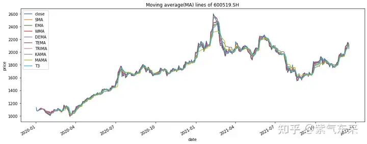
计算EMA
# EMA
N=[5,30,120,250]
for i in N:
    df['ma_'+str(i)]=ta.EMA(df.close,timeperiod=i)

df.loc['2021-01-01':,['close','ma_5','ma_30','ma_120','ma_250']].plot(figsize=(16,6),title='Exponential Moving Average(EMA) lines', xlabel='date', ylabel='price')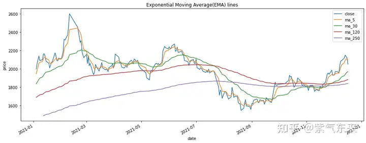
计算布林带
布林带(Bollinger Bands)由约翰·布林先生创造,其利用统计原理,求出股价的标准差及其信赖区间,从而确定股价的波动范围及未来走势,利用波带显示股价的安全高低价位。其上下限范围不固定,随股价的滚动而变化。布林指标属于路径指标,股价波动在上限和下限的区间之内,这条带状区的宽窄,随着股价波动幅度的大小而变化,股价涨跌幅度加大时,带状区变宽,涨跌幅度狭小盘整时,带状区则变窄。
- 中轨线 = N日的移动平均线
- 上轨线 = 中轨线 + K倍的标准差
- 下轨线 =中轨线 - K倍的标准差(K为参数,一般默认为2)
- 股价高于这个波动区间,即突破阻力线,说明股价虚高,卖出信号
- 股价低于这个波动区间,即跌破支撑线,说明股价虚低,买入信号
# BBANDS
H_line,M_line,L_line=ta.BBANDS(df.close, timeperiod=20, nbdevup=2, nbdevdn=2, matype=0)
df1=pd.DataFrame(df.close,index=df.index,columns=['close'])
df1['H_line']=H_line
df1['M_line']=M_line
df1['L_line']=L_line

df1.loc['2021-01-01':].plot(figsize=(16,6),title='Bollinger Bands', xlabel='date', ylabel='price')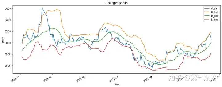
Momentum Indicators(动量指标类)
ADX                  Average Directional Movement Index(平均趋向指数)
ADXR                 Average Directional Movement Index Rating
APO                  Absolute Price Oscillator
AROON                Aroon
AROONOSC             Aroon Oscillator
BOP                  Balance Of Power
CCI                  Commodity Channel Index
CMO                  Chande Momentum Oscillator
DX                   Directional Movement Index
MACD                 Moving Average Convergence/Divergence (平滑异同移动平均线)
MACDEXT              MACD with controllable MA type
MACDFIX              Moving Average Convergence/Divergence Fix 12/26
MFI                  Money Flow Index
MINUS_DI             Minus Directional Indicator
MINUS_DM             Minus Directional Movement
MOM                  Momentum
PLUS_DI              Plus Directional Indicator
PLUS_DM              Plus Directional Movement
PPO                  Percentage Price Oscillator
ROC                  Rate of change : ((price/prevPrice)-1)*100
ROCP                 Rate of change Percentage: (price-prevPrice)/prevPrice
ROCR                 Rate of change ratio: (price/prevPrice)
ROCR100              Rate of change ratio 100 scale: (price/prevPrice)*100
RSI                  Relative Strength Index (相对强弱指数)
STOCH                Stochastic
STOCHF               Stochastic Fast
STOCHRSI             Stochastic Relative Strength Index
TRIX                 1-day Rate-Of-Change (ROC) of a Triple Smooth EMA
ULTOSC               Ultimate Oscillator
WILLR                Williams' %R
计算MACD
MACD的原理介绍参见
df['macd'], df['macdsignal'], df['macdhist'] = ta.MACD(df.close, fastperiod=12, slowperiod=26, signalperiod=9)
df[['close','macd','macdsignal','macdhist']].plot(figsize=(16,8),title='MACD', xlabel='date', ylabel='price')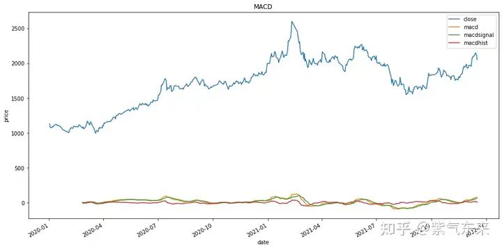
计算RSI
相对强弱指标(RSI)是根据股票市场上供求关系平衡的原理,通过比较一段时期内单个股票价格的涨跌的幅度或整个市场的指数的涨跌的大小来分析判断市场上多空双方买卖力量的强弱程度,从而判断未来市场走势的一种技术指标。
计算方法
N日RS=[A÷B]×100%
公式中,A——N日内收盘涨幅之和
B——N日内收盘跌幅之和(取正值)
N日 RSI = A/(A+B)×100
RSI的变动范围在0—100之间,强弱指标值一般分布在20—80。RSI值市场特征投资操作:
80—100极强卖出
50—80强买入
20—50弱观望
0—20极弱买入
代码实现:
df["rsi"] = ta.RSI(df.close, timeperiod=14)
ax = df[["close","rsi"]].plot(secondary_y=['rsi'],figsize=(16,8),title='RSI',xlabel='date', ylabel='price')
ax.right_ax.plot(df.index, [80]*len(df), '-', color='r')
ax.right_ax.plot(df.index, [20]*len(df), '-', color='r')
ax.right_ax.set_ylabel('%')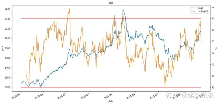
Volume Indicators(交易量指标)
AD                   Chaikin A/D Line
ADOSC                Chaikin A/D Oscillator
OBV                  On Balance Volume (能量潮)
计算OBV
能量潮指标(On Balance Volume,OBV)是葛兰维(Joe Granville)于上世纪60年代提出的,并被广泛使用,算是比较冷门的指标,虽然冷门,但是却威力巨大!股市技术分析的四大要素:价、量、时、空。OBV指标就是从“量”这个要素作为突破口,来发现热门股票、分析股价运动趋势的一种技术指标。它是将股市的人气—成交量与股价的关系数字化、直观化,以股市的成交量变化来衡量股市的推动力,从而研判股价的走势。关于成交量方面的研究,OBV能量潮指标是一种相当重要的分析指标之一。
计算公式:
当日OBV=前一日OBV+今日成交量
需要注意的是,如果当日收盘价高于前日收盘价取正值,反之取负值,平盘取零。- 当股价上升而OBV线下降,表示买盘无力,股价可能会回跌。
- 股价下降时而OBV线上升,表示买盘旺盛,逢低接手强股,股价可能会止跌回升。
代码实现:
obvta = ta.OBV(df['close'], df['vol'])
obv=[]
for i in range(0,len(df)):
    if i == 0:
        obv.append(df['vol'].values[i])
    else:
        if df['close'].values[i]>df['close'].values[i-1]:
            obv.append(obv[-1]+df['vol'].values[i])
        if df['close'].values[i]<df['close'].values[i-1]:
            obv.append(obv[-1]-df['vol'].values[i])
        if df['close'].values[i]==df['close'].values[i-1]:
            obv.append(obv[-1])
df['obv'] = obv
ax1 = df[["close","obv"]].plot(secondary_y=['obv'],figsize=(16,8),title='OBV',xlabel='date', ylabel='price')
ax1.right_ax.set_ylabel('OBV')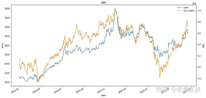
Price Transform(价格变换)
AVGPRICE             Average Price
MEDPRICE             Median Price
TYPPRICE             Typical Price
WCLPRICE             Weighted Close Price
计算各种价格
#开盘价,最高价,最低价,收盘价的均值
df['average']=ta.AVGPRICE(df.open,df.high,df.low,df.close)
#最高价,最低价的均值
df['median']=ta.MEDPRICE(df.high,df.low)
#最高价,最低价,收盘价的均值
df['typical']=ta.TYPPRICE(df.high,df.low,df.close)
#最高价,最低价,收盘价的加权
df['weight']=ta.WCLPRICE(df.high,df.low,df.close)
df.loc['2021-01-01':,['close','average','median','typical','weight']].plot(figsize=(16,8),title='Price Transform', xlabel='date', ylabel='price')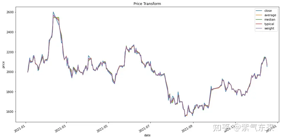

基于上述两条性质,我们可以分别采用
作为实轴、作为虚轴,构造正交复平面。
希尔伯特变换可实现价格序列瞬时信号的提取。
HT_DCPERIOD          Hilbert Transform - Dominant Cycle Period(希尔伯特变换-主导周期)
HT_DCPHASE           Hilbert Transform - Dominant Cycle Phase(希尔伯特变换-主导循环阶段)
HT_PHASOR            Hilbert Transform - Phasor Components(希尔伯特变换-相位构成)
HT_SINE              Hilbert Transform - SineWave(希尔伯特变换-正弦波)
HT_TRENDMODE         Hilbert Transform - Trend vs Cycle Mode(希尔伯特变换-趋势与周期模式)
计算方式如下:
df['dcperiod']=ta.HT_DCPERIOD(df.close)
df['dcphase']=ta.HT_DCPHASE(df.close)
df['inhpase'],df['quadrature']=ta.HT_PHASOR(df.close)
df['sine'],df['leadsine']=sine, leadsine = ta.HT_SINE(df.close)
df['trendmode']=ta.HT_TRENDMODE(df.close)

df[['close','dcperiod','dcphase','inhpase','quadrature','sine','leadsine','trendmode']].plot(figsize=(20,18),
       subplots = True,layout=(4, 2))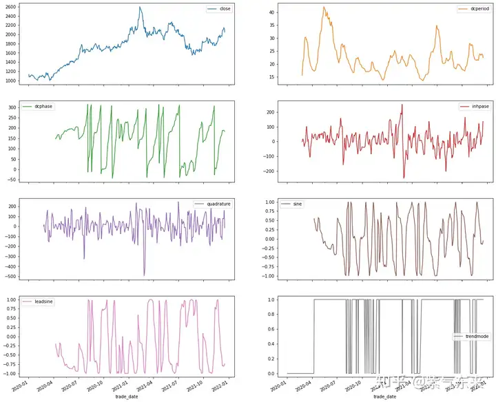
Volatility Indicators(波动率指标)
ATR                  Average True Range
NATR                 Normalized Average True Range
TRANGE               True Range
计算如下:
df['atr']=ta.ATR(df.high, df.low, df.close, timeperiod=14)
df['natr']=ta.NATR(df.high, df.low, df.close, timeperiod=14)
df['trange']=ta.TRANGE(df.high, df.low, df.close)

df[['close','atr','natr','trange']].plot(figsize=(16,10),subplots = True,layout=(2, 2))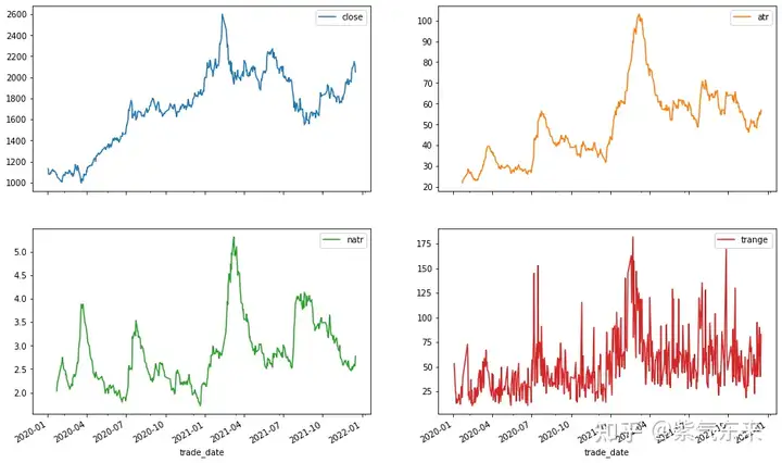
Math Operators(数学运算)
ADD                  Vector Arithmetic Add
DIV                  Vector Arithmetic Div
MAX                  Highest value over a specified period
MAXINDEX             Index of highest value over a specified period
MIN                  Lowest value over a specified period
MININDEX             Index of lowest value over a specified period
MINMAX               Lowest and highest values over a specified period
MINMAXINDEX          Indexes of lowest and highest values over a specified period
MULT                 Vector Arithmetic Mult
SUB                  Vector Arithmetic Substraction
SUM                  Summation
计算如下:
df['add']=ta.ADD(df.high,df.low)
df['sub']=ta.SUB(df.high,df.low)
df['mult']=ta.MULT(df.high,df.low)
df['div']=ta.DIV(df.high,df.low)
df['sum']=ta.SUM(df.close, timeperiod=30)
df['min'], df['max'] = ta.MINMAX(df.close, timeperiod=30)
#收盘价的每30日内的最大最小值对应的索引值(第N行)
df['minidx'], df['maxidx'] = ta.MINMAXINDEX(df.close, timeperiod=30)

df[['close','add','sub','mult','div','sum','min','max']].plot(figsize=(20,18), subplots = True, layout=(4, 2))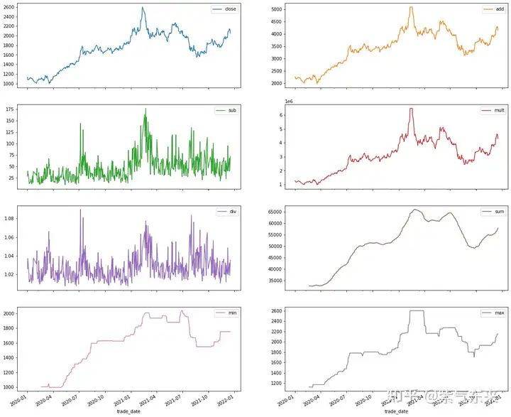
Statistic Functions(统计函数)
BETA                 Beta (贝塔系数)
CORREL               Pearson's Correlation Coefficient (r) (皮尔逊相关系数)
LINEARREG            Linear Regression
LINEARREG_ANGLE      Linear Regression Angle(线性回归正切角)
LINEARREG_INTERCEPT  Linear Regression Intercept(线性回归截距)
LINEARREG_SLOPE      Linear Regression Slope(线性回归斜率)
STDDEV               Standard Deviation
TSF                  Time Series Forecast(时序预测)
VAR                  Variance
计算如下:
df['linearreg']=ta.LINEARREG(df.close, timeperiod=14)
df['tsf']=ta.TSF(df.close, timeperiod=14)
df.loc['2021-08-01':,['close','linearreg','tsf']].plot(figsize=(12,6))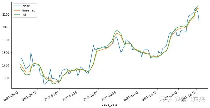
df['beta']=ta.BETA(df.high,df.low,timeperiod=5)
df['correl']=ta.CORREL(df.high, df.low, timeperiod=30)
df['stdev']=ta.STDDEV(df.close, timeperiod=5, nbdev=1)

df[['close','beta','correl','stdev']].plot(figsize=(18,8),subplots = True,layout=(2, 2))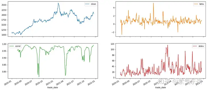
Math Transform(数学变换)
ACOS                 Vector Trigonometric ACos
ASIN                 Vector Trigonometric ASin
ATAN                 Vector Trigonometric ATan
CEIL                 Vector Ceil
COS                  Vector Trigonometric Cos
COSH                 Vector Trigonometric Cosh
EXP                  Vector Arithmetic Exp
FLOOR                Vector Floor
LN                   Vector Log Natural
LOG10                Vector Log10
SIN                  Vector Trigonometric Sin
SINH                 Vector Trigonometric Sinh
SQRT                 Vector Square Root
TAN                  Vector Trigonometric Tan
TANH                 Vector Trigonometric Tanh
计算如下:
df['sin']=ta.SIN(df.close)
df['cos']=ta.COS(df.close)
df['ln']=ta.LN(df.close)
df[['close','sin','cos','ln']].plot(figsize=(18,8),subplots = True,layout=(2, 2))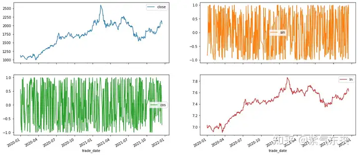

 浙公网安备 33010602011771号