强化学习导论 课后习题参考 - Chapter 5,6

Reinforcement Learning: An Introduction (second edition) - Chapter 5,6

Contents

• Chapter 1,2
• Chapter 3,4
• Chapter 5,6
• Chapter 7,8
• Chapter 9,10
• Chapter 11,12,13

Chapter 5

5.1
Consider the diagrams on the right in Figure 5.1. Why does the estimated value function jump up for the last two rows in the rear? Why does it drop off for the whole last row on the left? Why are the frontmost values higher in the upper diagrams than in the lower?

• 游戏规则不熟，只能说点感觉上的东西。最后两行手牌已经是20、21，是所有排里很大的牌了，估计值高也很正常。关键这个jump，为什么19不高，18不高？主要是这里的策略是在20,21就停手（sticks），其他策略继续要牌（hits），就容易超过21，所以有一个jump的情形。左边低是因为庄家有一张A，这个又可以当1又可以当11，自然会增加专家赢牌的概率。上图比下图在前期的值更大，还是因为有A的原因，毕竟又可以当1又可以当11。

5.2
Suppose every-visit MC was used instead of first-visit MC on the blackjack task. Would you expect the results to be very different? Why or why not?

• 应该是没有影响的。因为当前状态可以表示之后策略所需的所有元素，和再之前的状态无关了，不管从什么状态到这个状态，之后的策略都是一样的，所以是不是first-visit没有区别。
• 一个episode里不会有两个相同的状态。

5.3
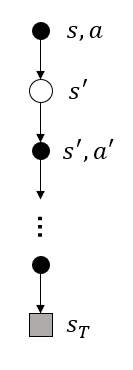
What is the backup diagram for Monte Carlo estimation of \(q_\pi\)?

• 把\(s,a\)画前面

5.4
The pseudocode for Monte Carlo ES is inefficient because, for each state–action pair, it maintains a list of all returns and repeatedly calculates their mean. It would be more efficient to use techniques similar to those explained in Section 2.4 to maintain just the mean and a count (for each state–action pair) and update them incrementally. Describe how the pseudocode would be altered to achieve this.

• Initialize部分，初始化一个计数\(N(s,a)\leftarrow 0, \text{for all} \ s \in \mathcal{S}, a \in \mathcal{A}(s)\)，把return的list直接不要了。
• 在伪代码里把\(\text{Append} \ G \ to \ Returns(S_t,A_t); \ Q(S_t,A_t)\leftarrow\text{average}(Returns(S_t,A_t))\)改成\(N(S_t,A_t)\leftarrow N(S_t,A_t)+1; \ Q(S_t,A_t) \leftarrow Q(S_t,A_t)+\frac{1}{N(S_t,A_t)}(G-Q(S_t,A_t))\)。

5.5
Consider an MDP with a single nonterminal state and a single action that transitions back to the nonterminal state with probability \(p\) and transitions to the terminal state with probability \(1−p\). Let the reward be +1 on all transitions, and let \(\gamma=1\). Suppose you observe one episode that lasts 10 steps, with a return of 10. What are the first-visit and every-visit estimators of the value of the nonterminal state?

• first-visit只算第一次的，所以这条轨迹就是这个状态的估计，有\(v_{first-visit}(s)=10\)。every-visit是每到这个状态就会算一条轨迹的return，总共经历了10次，每次的return都通过\(G_t=\sum_{k=t+1}^T\gamma^{k-t-1} R_k\)计算， 每次的\(G_t\)分别是\(10,9,8,...,2,1\)。所以有\(v_{every-visit}(s)=\frac{10+9+...+1}{10}=5.5\)。

5.6 What is the equation analogous to (5.6) for action values \(Q(s, a)\) instead of state values \(V(s)\), again given returns generated using \(b\)?

• 这个地方先仿照式(5.4)把\(q_\pi\)写出来。有\(E[\rho_{t+1:T-1}G_t|S_t=s,A_t=a]=q_\pi(s,a)\)，注意这里\(\rho\)是从\(t+1\)开始的，因为从前面的定义有

\[\rho_{t:T-1} \overset{.}{=} \prod_{k=t}^{T-1}\frac{\pi(A_k|S_k)}{b(A_k|S_k)} \]

因为\(q_\pi(s,a)\)已经把\(S_k\)下\(A_k\)选过了，所以只用决定\(t+1\)之后的动作序列。此外，之前定义的\(\mathcal{T}(s)\)是只包含状态的时刻表示，改为包含动作的\(\mathcal{T}(s,a)\)，最终有

\[Q(s,a)=\frac{\sum_{t+1 \in \mathcal{T(s,a)}}\rho_{t+1:T-1}G_t}{|\mathcal{T}(s,a)|} \]

5.7
In learning curves such as those shown in Figure 5.3 error generally decreases with training, as indeed happened for the ordinary importance-sampling method. But for the weighted importance-sampling method error first increased and then decreased. Why do you think this happened?

• 可能是因为ordinary importance-sampling方差大，weighted importance-sampling方差小，所以ordinary importance-sampling刚开始误差大，曲线在上面。而weighted刚开始小，中间又上升，可能是没有采样到这个状态，所以还是初始值0，碰巧误差比较小。中间随着采样，先略微上升，再误差减小。不过也有可能是因为weighted importance-sampling是有偏的，偏差造成了误差刚开始变大了，随着采样增加，偏差减少，误差也减少。

5.8
The results with Example 5.5 and shown in Figure 5.4 used a first-visit MC method. Suppose that instead an every-visit MC method was used on the same problem. Would the variance of the estimator still be infinite? Why or why not?

• first-visit MC method里面，只算第一次访问，先按书本里的写出来

\[\begin{array}{l} E[X^2]= \frac{1}{2} \cdot 0.1(\frac{1}{0.5})^2 \\ \\ \ \qquad \quad \ + \frac{1}{2} \cdot 0.9\cdot\frac{1}{2} \cdot 0.1(\frac{1}{0.5}\frac{1}{0.5})^2 \\ \\ \ \qquad \quad \ + \frac{1}{2} \cdot 0.9\cdot\frac{1}{2} \cdot 0.9\cdot\frac{1}{2} \cdot 0.1(\frac{1}{0.5}\frac{1}{0.5}\frac{1}{0.5})^2 \\ \\ \ \qquad \quad \ + \cdots \\ \\ \qquad \quad \ = 0.1\sum_{k=0}^{\infty}0.9^k\cdot2^k\cdot2 = 0.2 \sum_{k=0}^{\infty}1.8^k=\infty \end{array} \]

根据上面这个式子，把多次访问的序列拆成every-visit的形式，计算平均。比如长度1的序列不变，长度为2的序列计算两次，长度为3的序列计算3次，以此类推。

\[\begin{array}{l} E[X^2]= \frac{1}{2} \cdot 0.1(\frac{1}{0.5})^2 \\ \ \qquad \quad \ + \frac{1}{2} \cdot 0.9\cdot\frac{1}{2} \cdot 0.1[(\frac{1}{0.5})^2+(\frac{1}{0.5}\frac{1}{0.5})^2]/2\\ \ \qquad \quad \ + \frac{1}{2} \cdot 0.9\cdot\frac{1}{2} \cdot 0.9\cdot\frac{1}{2} \cdot 0.1[(\frac{1}{0.5})^2+(\frac{1}{0.5}\frac{1}{0.5})^2+(\frac{1}{0.5}\frac{1}{0.5}\frac{1}{0.5})^2]/3 \\ \ \qquad \quad \ + \cdots \\ \\ \qquad \quad \ > \frac{1}{2} \cdot 0.1(\frac{1}{0.5})^2 \\ \ \qquad \quad \ + \frac{1}{2} \cdot 0.9\cdot\frac{1}{2} \cdot 0.1[(\frac{1}{0.5}\frac{1}{0.5})^2]/2 \\ \ \qquad \quad \ + \frac{1}{2} \cdot 0.9\cdot\frac{1}{2} \cdot 0.9\cdot\frac{1}{2} \cdot 0.1[(\frac{1}{0.5}\frac{1}{0.5}\frac{1}{0.5})^2]/3 \\ \ \qquad \quad \ + \cdots \\ \\ \qquad \quad \ > \frac{1}{2} \cdot 0.1(\frac{1}{0.5})^2 \\ \ \qquad \quad \ + \frac{1}{2} \cdot 0.1[(\frac{1}{0.5})^2]/2 \\ \ \qquad \quad \ + \frac{1}{2} \cdot 0.1[(\frac{1}{0.5})^2]/3 \\ \ \qquad \quad \ + \cdots \\ \\ \qquad \quad= \frac{1}{2} \cdot 0.1\cdot(\frac{1}{0.5})^2[1+\frac{1}{2}+\frac{1}{3}+\cdots] =\infty \end{array} \]

所以也是无穷的。
之前我一直在想需不需要平均，是不是加起来就行了。后来觉得，既然是期望，那么去掉ratio和return部分，关于概率的积分应该为1才行，比如every-visit里面每条轨迹出现的概率之和为1。如果不平均，那不是相当于这条轨迹出现的概率增加了，所以还是除以一下把后面的值算到轨迹的平均值里可能更说得通。

5.9
Modify the algorithm for first-visit MC policy evaluation (Section 5.1) to use the incremental implementation for sample averages described in Section 2.4.

• 和Excercise 5.4类似，Initialize部分，初始化一个计数\(N(s)\leftarrow 0, \text{for all} \ s \in \mathcal{S}\)，把return的list直接不要了。
• 在伪代码里把\(\text{Append} \ G \ to \ Returns(S_t); \ V(S_t)\leftarrow\text{average}(Returns(S_t))\)改成\(N(S_t)\leftarrow N(S_t)+1; \ V(S_t) \leftarrow V(S_t)+\frac{1}{N(S_t)}(G-V(S_t))\)。

5.10
Derive the weighted-average update rule (5.8) from (5.7). Follow the pattern of the derivation of the unweighted rule (2.3).

• 拆开凑一下

\[\begin{array}{l} V_{n+1} = \frac{\sum_{k=1}^nW_kG_k}{\sum_{k=1}^nW_k} \\ \\ = \frac{\sum_{j=1}^{n-1}W_j\sum_{k=1}^nW_kG_k}{\sum_{j=1}^{n-1}W_j\sum_{k=1}^nW_k} \\ \\ = \frac{\sum_{j=1}^{n}W_j\sum_{k=1}^nW_kG_k-W_n\sum_{k=1}^nW_kG_k}{\sum_{j=1}^{n-1}W_j\sum_{k=1}^nW_k} \\ \\ = \frac{\sum_{j=1}^{n}W_j(\sum_{k=1}^{n-1}W_kG_k+W_nG_n)-W_n\sum_{k=1}^nW_kG_k}{\sum_{j=1}^{n-1}W_j\sum_{k=1}^nW_k} \\ \\ = \frac{\sum_{j=1}^{n}W_j\sum_{k=1}^{n-1}W_kG_k+W_nG_n\sum_{j=1}^{n}W_j-W_n\sum_{k=1}^nW_kG_k}{\sum_{j=1}^{n-1}W_j\sum_{k=1}^nW_k} \\ \\ = \frac{\sum_{j=1}^{n}W_j\sum_{k=1}^{n-1}W_kG_k}{\sum_{j=1}^{n-1}W_j\sum_{k=1}^nW_k} + \frac{W_nG_n\sum_{j=1}^{n}W_j-W_n\sum_{k=1}^nW_kG_k}{\sum_{j=1}^{n-1}W_j\sum_{k=1}^nW_k} \\ \\ = \frac{\sum_{k=1}^{n-1}W_kG_k}{\sum_{j=1}^{n-1}W_j} + \frac{W_n}{\sum_{k=1}^nW_k}\frac{G_n\sum_{j=1}^{n}W_j-\sum_{k=1}^nW_kG_k}{\sum_{j=1}^{n-1}W_j} \\ \\ = \frac{\sum_{k=1}^{n-1}W_kG_k}{\sum_{j=1}^{n-1}W_j} + \frac{W_n}{\sum_{k=1}^nW_k}\frac{G_n\sum_{j=1}^{n-1}W_j-\sum_{k=1}^{n-1}W_kG_k}{\sum_{j=1}^{n-1}W_j} \\ \\ = V_n + \frac{W_n}{C_n}[G_n-V_n] \end{array} \]

5.11
In the boxed algorithm for off-policy MC control, you may have been expecting the \(W\) update to have involved the importance-sampling ratio \(\frac{\pi(A_t|S_t)}{b(A_t|S_t)}\), but instead it involves \(\frac{1}{b(A_t|S_t)}\). Why is this nevertheless correct?

• 因为这里的\(\pi\)是greedy策略，被选动作的概率为1，所以直接写成\(\frac{1}{b(A_t|S_t)}\)了。

5.12:
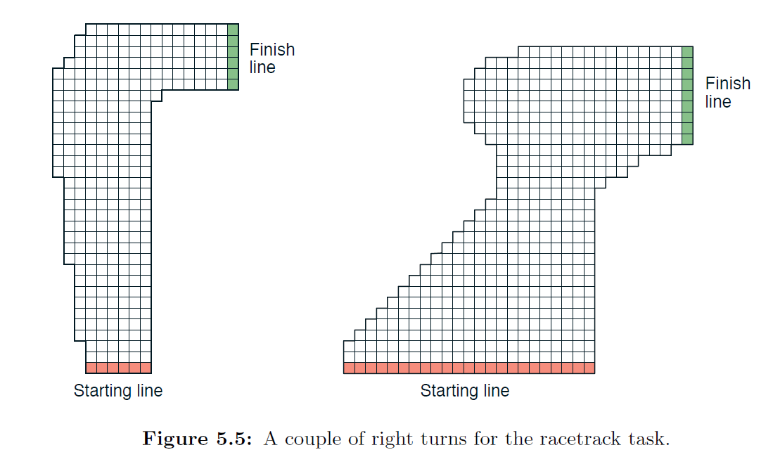
Racetrack (programming) Consider driving a race car around a turn like those shown in Figure 5.5. You want to go as fast as possible, but not so fast as to run off the track. In our simplified racetrack, the car is at one of a discrete set of grid positions, the cells in the diagram. The velocity is also discrete, a number of grid cells moved horizontally and vertically per time step. The actions are increments to the velocity components. Each may be changed by +1, −1, or 0 in each step, for a total of nine (3x3) actions. Both velocity components are restricted to be nonnegative and less than 5, and they cannot both be zero except at the starting line. Each episode begins in one of the randomly selected start states with both velocity components zero and ends when the car crosses the finish line. The rewards are −1 for each step until the car crosses the finish line. If the car hits the track boundary, it is moved back to a random position on the starting line, both velocity components are reduced to zero, and the episode continues. Before updating the car’s location at each time step, check to see if the projected path of the car intersects the track boundary. If it intersects the finish line, the episode ends; if it intersects anywhere else, the car is considered to have hit the track boundary and is sent back to the starting line. To make the task more challenging, with probability 0.1 at each time step the velocity increments are both zero, independently of the intended increments. Apply a Monte Carlo control method to this task to compute the optimal policy from each starting state. Exhibit several trajectories following the optimal policy (but turn the noise off for these trajectories).

5.13
Show the steps to derive (5.14) from (5.12).

• 首先要说明\(R_{t+1}\)只和\(S_t,A_t\)有关，而和后面的状态动作序列无关，所以可以把期望都拆开，只剩第一项。

\[\begin{array}{l} E[\rho_{t:T-1}R_t] = E_b[\frac{\pi(A_t|S_t)}{b(A_t|S_t)}\frac{\pi(A_{t+1}|S_{t+1})}{b(A_{t+1}|S_{t+1})}\cdots\frac{\pi(A_{T-1}|S_{T-1})}{b(A_{T-1}|S_{T-1})}R_{t+1}] \\ \\ = E_b[\frac{\pi(A_t|S_t)}{b(A_t|S_t)}R_{t+1}]E_b[\frac{\pi(A_{t+1}|S_{t+1})}{b(A_{t+1}|S_{t+1})}]\cdots E_b[\frac{\pi(A_{T-1}|S_{T-1})}{b(A_{T-1}|S_{T-1})}] \\ \\ = E_b[\frac{\pi(A_t|S_t)}{b(A_t|S_t)}R_{t+1}] \\ \\ = E[\rho_{t:t}R_{t+1}] \end{array} \]

5.14
Modify the algorithm for off-policy Monte Carlo control (page 111) to use the idea of the truncated weighted-average estimator (5.10). Note that you will first need to convert this equation to action values.

• 想了半天，也没想到一个可以一个循环，只维护几个数的写法，感觉要维护几个list才行，要降低运算，就用numpy的形式。最终维护三个array，每个都是长度为T的一维数组，分别表示\(\bar G,\rho,\Gamma\)的变化。
• 需要记住几个定义：

\[\bar G_{t:h} \overset{.}{=}R_{t+1}+R_{t+2}+\cdots+R_{h}, 0 \leq t<h\leq T \]

\[G_t = (1-\gamma)\sum^{T+1}_{h=t+1}\gamma^{h-t-1}\bar G_{t:h}+\gamma^{T-t-1}\bar G_{t:T} \]

\[\rho_{t:T-1} = \prod_{k=t}^{T-1}\frac{\pi(A_k|S_k)}{b(A_k|S_k)} \]

\[V(s) \overset{.}{=} \frac{\sum_{t \in \mathcal{T}(s)}((1-\gamma)\sum^{T(t)-1}_{h=t+1}\gamma^{h-t-1}\rho_{t:h-1}\bar G_{t:h}+\gamma^{T(t)-t-1}\rho_{t:T(t)-1}\bar G_{t:T(t)})}{|\mathcal{T}(s)|} \]

\[Q(s,a) \overset{.}{=} \frac{\sum_{t \in \mathcal{T}(s,a)}((1-\gamma)\sum^{T(t)-1}_{h=t+1}\gamma^{h-t-1}\rho_{t+1:h-1}\bar G_{t:h}+\gamma^{T(t)-t-1}\rho_{t+1:T(t)-1}\bar G_{t:T(t)})}{|\mathcal{T}(s,a)|} \]

• 这里把里面的loop人工写一遍，注意这里更新的是\(Q(s,a)\)，所以同Excercise 5.6，\(\rho\)要从t+1开始算起，即\(\rho_{t+1:h-1}\)，其中若\(t+1>h-1\)，则\(\rho_{t+1:h-1}=1\)。然后计算的\(Q(s,a)\)的每一项可以表示为\(Q(s,a)=(1-\gamma) \cdot\text{sum} (\Gamma[:-1] \cdot \rho[:-1] \cdot \bar G[:-1])+ \Gamma[-1] \cdot\rho[-1] \cdot \bar G[-1]\)，也就是\(Q(s,a)\)中的\((1-\gamma)\sum^{T(t)-1}_{h=t+1})\gamma^{h-t-1}\rho_{t+1:h-1}\bar G_{t:h}+\gamma^{T(t)-t-1}\rho_{t+1:T(t)-1}\bar G_{t:T(t)})\)。注意这里的乘都是numpy的运算，对应位置相乘。简写\(T(t)\)为\(T\)。整个示例如下：

t	r & b	\(\bar G\)	\(\rho\)	\(\Gamma\)	结果 G & W
-	-	\([0,\cdots,0]\)	\([0,\cdots,0]\)	\([0,\cdots,0]\)	-
\(T-1\)	\(R_T\) 1	\([0,\cdots,0,\bar G_{T-1:T}]\)	\([0,\cdots,0,1]\)	\([0,\cdots,0,1]\)	\(\bar G_{T-1:T}\) \(1\)
\(T-2\)	\(R_{T-1}\) \(b(A_{T-1}|S_{T-1})\)	\([\cdots,\bar G_{T-2:T-1},\bar G_{T-2:T}]\)	\([0,\cdots,1,\rho_{T-1:T-1}]\)	\([0,\cdots,1,\gamma]\)	\((1-\gamma)\sum^{T-1}_{h=T-1}\gamma^{h-T+1}\rho_{T-1:h-1}\bar G_{T-2:h}+\gamma \rho_{T-1:T-1}\bar G_{T-1:T})\) \((1-\gamma)\sum^{T-1}_{h=T-1}\gamma^{h-T+1}\rho_{T-1:h-1}+\gamma \rho_{T-1:T-1})\)
\(T-3\)	\(R_{T-2}\) \(b(A_{T-2}|S_{T-2})\)	\([\cdots,\bar G_{T-3:T-2},\bar G_{T-3:T-1},\bar G_{T-3:T}]\)	\([\cdots,1,\rho_{T-2:T-2},\rho_{T-2:T-1}]\)	\([\cdots,1,\gamma,\gamma^2]\)	\((1-\gamma)\sum^{T-1}_{h=T-2}\gamma^{h-T+2}\rho_{T-2:h-1}\bar G_{T-3:h}+\gamma^{2}\rho_{T-2:T-1}\bar G_{T-3:T})\) \((1-\gamma)\sum^{T-1}_{h=T-2}\gamma^{h-T+2}\rho_{T-2:h-1}+\gamma^{2}\rho_{T-2:T-1})\)
...	...	...	...	...	...

• 现在需要的就是把表里的每一行转成代码，每次新来一个\(R,b\)，就更新\(\bar G , \rho , \Gamma\)

\[\begin{array}{l} \bar G \leftarrow (\bar G != 0)\cdot R_{t+1} + \bar G \\ \bar G[t] \leftarrow R_{t+1} \\ \rho \leftarrow (\rho != 0)\cdot \frac{1}{b(A_t|S_t)} \cdot \rho \\ \rho \leftarrow 1 \\ \Gamma \leftarrow (\Gamma != 0)\cdot \gamma \cdot \Gamma \\ \Gamma[t] \leftarrow 1 \end{array} \]

• 整个过程结束。可能有更简单的写法，再想想。

---

Chapter 6

6.1
If \(V\) changes during the episode, then (6.6) only holds approximately; what would the difference be between the two sides? Let \(V_t\) denote the array of state values used at time \(t\) in the TD error (6.5) and in the TD update (6.2). Redo the derivation above to determine the additional amount that must be added to the sum of TD errors in order to equal the Monte Carlo error.

• 这个题因为之前书上是简写的记号，所以理解了半天什么意思。其实是想和更新的时刻联系起来。首先这里是tabular的情形，其次更新公式\(V(S_t)\leftarrow V(S_t) + \alpha[R_{t+1}+\gamma V(S_{t+1})-V(S_t)]\)实际上应该写成

\[V_{t+1}(S_t)\leftarrow V_{t}(S_t) + \alpha[R_{t+1}+\gamma V_{t}(S_{t+1})-V_{t}(S_t)] \]

所以\(\delta_t\)都写成和更新时刻\(t\)相关的式子：

\[\begin{array}{l} \delta_t \overset{.}{=}R_{t+1}+\gamma V_{t}(S_{t+1})-V_{t}(S_t) \\ \\ \delta_{t+1} \overset{.}{=}R_{t+2}+\gamma V_{t+1}(S_{t+2})-V_{t+1}(S_{t+1}) \\ \\ \delta_{t+2} \overset{.}{=}R_{t+3}+\gamma V_{t+2}(S_{t+3})-V_{t+2}(S_{t+2}) \\ \\ \cdots\cdots \end{array} \]

题目就是说之前\(\delta_t\)没有区别这个地方，改成这个形式，如下：

\[\begin{array}{l} G_t-V_t(S_t)=R_{t+1}+\gamma G_{t+1} -V_t(S_t)+\gamma V_t(S_{t+1})-\gamma V_t(S_{t+1}) \\ \\ \qquad \qquad\quad \ = R_{t+1}+\gamma V_{t}(S_{t+1})-V_{t}(S_t) + \gamma(G_{t+1}-V_t(S_{t+1})) \\ \\ \qquad \qquad\quad \ =\delta_t+\gamma(G_{t+1}-V_t(S_{t+1})) \\ \\ \qquad \qquad\quad \ =\delta_t+\gamma(G_{t+1}-V_{t+1}(S_{t+1})+V_{t+1}(S_{t+1})-V_t(S_{t+1})) \\ \\ \qquad \qquad\quad \ =\delta_t+\gamma(G_{t+1}-V_{t+1}(S_{t+1}))+\gamma(V_{t+1}(S_{t+1})-V_t(S_{t+1})) \\ \\ \qquad \qquad\quad \ =\delta_t+\gamma(\delta_{t+1}+\gamma(G_{t+2}-V_{t+2}(S_{t+2}))+\gamma(V_{t+2}(S_{t+2})-V_{t+1}(S_{t+2})))+\gamma(V_{t+1}(S_{t+1})-V_t(S_{t+1})) \\ \\ \qquad \qquad\quad \ = \delta_t+\gamma\delta_{t+1}+\gamma^2(G_{t+2}-V_{t+2}(S_{t+2}))+\gamma^2(V_{t+2}(S_{t+2})-V_{t+1}(S_{t+2}))+\gamma(V_{t+1}(S_{t+1})-V_t(S_{t+1})) \\ \\ \qquad \qquad\quad \ \cdots \\ \\ \qquad \qquad\quad \ = \sum_{k=t}^{T-1}\gamma^{k-t}\delta_{k} + \sum_{k=t}^{T-1}\gamma^{k-t+1}(V_{k+1}(S_{k+1})-V_{k}(S_{k+1})) \end{array} \]

6.2
This is an exercise to help develop your intuition about why TD methods are often more efficient than Monte Carlo methods. Consider the driving home example and how it is addressed by TD and Monte Carlo methods. Can you imagine a scenario in which a TD update would be better on average than a Monte Carlo update? Give an example scenario—a description of past experience and a current state—in which you would expect the TD update to be better. Here’s a hint: Suppose you have lots of experience driving home from work. Then you move to a new building and a new parking lot (but you still enter the highway at the same place). Now you are starting to learn predictions for the new building. Can you see why TD updates are likely to be much better, at least initially, in this case? Might the same sort of thing happen in the original scenario?

• 这个题的意思就是场景发生了部分改变，比如搬到了新地方。从新地方去上班，前面这段路是没见过的，但是上高速路了之后就和之前一样了。这种情形下，TD方法因为会利用下一步的估计值，相比于蒙特卡洛方法从头开始学起，肯定会收敛更快。

6.3
From the results shown in the left graph of the random walk example it appears that the first episode results in a change in only \(V(A)\). What does this tell you about what happened on the first episode? Why was only the estimate for this one state changed? By exactly how much was it changed?

• 说明第一个episode是在左边结束的，得到reward为0。根据更新公式

\[V(S_t)\leftarrow V(S_t) + \alpha[R_{t+1}+\gamma V(S_{t+1})-V(S_t)]=V(S_t) + 0.1\cdot[R_{t+1}+ V(S_{t+1})-V(S_t)] \]

对于其他状态，更新为\(V(S_t)\leftarrow V(S_t) + 0.1\cdot[0+ 0.5-0.5]\)值不变。对\(A\)有\(V(A)\leftarrow 0.5 + 0.1\cdot[0+ 0-0.5]=0.45\)。

6.4
The specific results shown in the right graph of the random walk example are dependent on the value of the step-size parameter, \(\alpha\). Do you think the conclusions about which algorithm is better would be affected if a wider range of \(\alpha\) values were used? Is there a different, fixed value of \(\alpha\) at which either algorithm would have performed significantly better than shown? Why or why not?

• 这个问题有点开放，不知道怎么回答。单从图上来看，TD对参数更加敏感，MC影响较小。具体有没有一个值对两个算法都好，估计要做实验试试了。这种问题感觉没有说哪个比哪个更好，都是有好有坏。比如 \(\alpha\) 小，收敛更慢但是更平稳更准确。\(\alpha\)小，收敛更快但是更加震荡效果更差。

6.5
In the right graph of the random walk example, the RMS error of the TD method seems to go down and then up again, particularly at high \(\alpha \text{'s}\). What could have caused this? Do you think this always occurs, or might it be a function of how the approximate value function was initialized?

• 震荡是不可避免的，因为这个过程是随机过程，每个episode的值都会有随机性，估计有方差。若\(\alpha\)大，方差更大，震荡就更厉害。另一方面，初始值没有影响，因为常数的加减不影响方差。

6.6
In Example 6.2 we stated that the true values for the random walk example
are \(\frac{1}{6},\frac{2}{6},\frac{3}{6},\frac{4}{6},\text{and} \ \frac{5}{6}\), for states A through E. Describe at least two different ways that these could have been computed. Which would you guess we actually used? Why?

• 一个是直接和例子一样，用强化的方法，比如MC和TD。另一个是用DP的方式直接计算贝尔曼方程。估计是用DP，这样可以直接解方程得到准确值，而且用\(v_\pi(C)=0.5\)可以简化很多计算。
• 同MDP中值函数的求解，贝尔曼方程可矩阵表示如下

\[v = R +\gamma Pv \]

则有

\[v = R +\gamma Pv\\ (I-\gamma P)v = R\\ v = (I - \gamma P)^{-1}R \]

直接写出矩阵解出来即可。有代码如下：

	import numpy as np  
	P =np.matrix([[0,0,0,0,0,0,0],  
	  [0.5,0,0.5,0,0,0,0],  
	  [0,0.5,0,0.5,0,0,0],  
	  [0, 0,0.5, 0, 0.5, 0, 0],  
	  [0, 0, 0,0.5, 0, 0.5, 0],  
	  [0,0,0,0,0.5,0,0.5],  
	  [0, 0, 0, 0, 0, 0,0]])  
	I = np.eye(7)  
	R = np.matrix([[0,0,0,0,0,1/2,0.]]).T  
	
	print(np.dot(np.linalg.inv(I-P),R))

得到\([0,\frac{1}{6},\frac{2}{6},\frac{3}{6},\frac{4}{6},\frac{5}{6},0]\)

• 如果用上\(v_\pi(C)=0.5\)，不用矩阵表示，直接列出每个状态之间的关系，会更快。比如\(v_\pi(E)=\frac{1}{2}\times1+\frac{1}{2}v_\pi(D)=\frac{1}{2}+\frac{1}{2}(\frac{1}{2}v_\pi(C)+\frac{1}{2}v_\pi(E))\)，得\(v_\pi(E)=\frac{5}{6}\)。其他同理。

6.7
Design an off-policy version of the TD(0) update that can be used with arbitrary target policy \(\pi\) and covering behavior policy \(b\), using at each step \(t\) the importance sampling ratio \(\rho_{t:t}\) (5.3).

• 先看最基本的更新式子(6.1)(6.2)

\[\begin{array}{l} V(S_t)\leftarrow V(S_t)+\alpha [G_t-V(S_t)] \qquad \qquad \qquad \qquad (6.1)\\ V(S_t)\leftarrow V(S_t)+\alpha [R_{t+1}+\gamma V(S_{t+1})-V(S_t)] \qquad (6.2) \end{array} \]

此时有\(v_\pi(s)=E_{\pi}[G_t|S_t=s]\)。
根据式子(5.4)现在有\(v_\pi(s)=E_b[\rho_{t:T-1}G_t|S_t=s]\)，其中数据来自\(b\)。所以要做的事情就是把\(G_t\)换成\(\rho_{t:T-1}G_t\)，所以(6.1)有\(V(S_t)\leftarrow V(S_t)+\alpha [\rho_{t:T-1}G_t-V(S_t)]\)。另一方面

\[\begin{array}{l} \rho_{t:T-1}G_t = \rho_{t:T-1}[R_{t+1}+\gamma G_{t+1}] \\ \qquad \quad \ \ \ = \rho_{t:T-1}R_{t+1}+ \rho_{t:T-1} \gamma G_{t+1} \\ \qquad \quad \ \ \ = \rho_{t:T-1}R_{t+1}+ \rho_{t:t} \gamma \rho_{t+1:T-1}G_{t+1} \\ \qquad \quad \ \ \ = \rho_{t:T-1}R_{t+1}+ \rho_{t:t} \gamma V(S_{t+1}) \\ \qquad \quad \ \ \ = \rho_{t:t}R_{t+1}+ \rho_{t:t} \gamma V(S_{t+1}) \qquad (E[\rho_{t:T-1}R_{t+1}]=E[\rho_{t:t}R_{t+1}] \cdots (5.14)) \end{array} \]

所以(6.2)有\(V(S_t)\leftarrow V(S_t)+\alpha [\rho_{t:t}R_{t+1}+ \rho_{t:t}\gamma V(S_{t+1})-V(S_t)]\)，即带重要性采样的TD(0)更新。

6.8
Show that an action-value version of (6.6) holds for the action-value form of the TD error (\(\delta_t =R_{t+1}+\gamma Q(S_{t+1},A_{t+1})-Q(S_t,A_t)\), again assuming that the values don’t change from step to step.

• 直接写

\[\begin{array}{l} G_t - Q(S_t,A_t)= R_{t+1} + \gamma G_{t+1} - Q(S_t,A_t) + \gamma Q(S_{t+1},A_{t+1}) - \gamma Q(S_{t+1},A_{t+1}) \\ \qquad \quad \quad \quad \quad \ \ \ = R_{t+1} + \gamma Q(S_{t+1},A_{t+1}) - Q(S_t,A_t)+ \gamma G_{t+1}- \gamma Q(S_{t+1},A_{t+1}) \\ \qquad \quad \quad \quad \quad \ \ \ = \delta_t + \gamma (G_{t+1}-Q(S_{t+1},A_{t+1})) \\ \qquad \quad \quad \quad \quad \ \ \ = \delta_t + \gamma \delta_{t+1} + \cdots + \gamma^{T-1} (G_T-Q(S_T,A_T)) \\ \qquad \quad \quad \quad \quad \ \ \ = \sum_{k=t}^{T-1}\gamma^{k-t}\delta_k \end{array} \]

6.9:
Windy Gridworld with King’s Moves (programming) Re-solve the windy gridworld assuming eight possible actions, including the diagonal moves, rather than the usual four. How much better can you do with the extra actions? Can you do even better by including a ninth action that causes no movement at all other than that caused by the wind?

6.10:
Stochastic Wind (programming) Re-solve the windy gridworld task with King’s moves, assuming that the effect of the wind, if there is any, is stochastic, sometimes varying by 1 from the mean values given for each column. That is, a third of the time you move exactly according to these values, as in the previous exercise, but also a third of the time you move one cell above that, and another third of the time you move one cell below that. For example, if you are one cell to the right of the goal and you move left, then one-third of the time you move one cell above the goal, one-third of the time you move two cells above the goal, and one-third of the time you move to the goal.

6.11
Why is Q-learning considered an off-policy control method?

• 关键区别就在于更新公式里的max操作。off-policy的定义是与环境交互的策略和学习的策略不是同一个策略。首先我们知道Q-learning与环境交互用的是\(\epsilon\)-greedy策略，而学习的策略由于max的存在，是greedy策略，两个策略不是同一个策略，所以是off-policy的。
• 这也是为什么在Example 6.6里Q-learning相较于Sarsa，在学习过程中更倾向于走更危险但是回报也会更高的地方，因为Q-learning学的时候是不考虑\(\epsilon\)的，只会去学最大值，而挨着悬崖的地方显然值更大。而在和环境交互学习的时候走这些地方就很有可能因为\(\epsilon\)的存在而突然走到悬崖得到-100，也就更危险。相反Sarsa在学习的时候也考虑了\(\epsilon\)，所以相对更加保守。

6.12 Suppose action selection is greedy. Is Q-learning then exactly the same algorithm as Sarsa? Will they make exactly the same action selections and weight updates?

• 如果选择动作变成greedy，那么Q-learning也是on-policy了，不过只能说是同一类算法，不能说是一样吧。两种方法得到的结果也不会一样，毕竟on-policy的方法必须要有探索才能保证每个状态被访问到无穷次，进而学到全局最优，显然Sarsa的效果会更好。

6.13
What are the update equations for Double Expected Sarsa with an \(\epsilon\)-greedy target policy?

• 写出Expected Sarsa的更新公式

\[Q(S_t,A_t) \leftarrow Q(S_t,A_t)+\alpha[R_{t+1}+\gamma \sum_a\pi(a|S_{t+1})Q(S_{t+1},a)-Q(S_t,A_t) ] \]

把Q换成两个，

\[Q_1(S_t,A_t) \leftarrow Q_1(S_t,A_t)+\alpha[R_{t+1}+\gamma \sum_a\pi_1(a|S_{t+1})Q_2(S_{t+1},a)-Q_1(S_t,A_t) ] \]

其中\(\pi(a|S_t)= \left\{\begin{array}{l} 1-\epsilon+\epsilon/|\mathcal{A}(S_t)|, \quad if \ a=A^*\\ \epsilon/|\mathcal{A}(S_t)|, \qquad \qquad \ if \ a \not = A^* \end{array}\right.\)

6.14
Describe how the task of Jack’s Car Rental (Example 4.2) could be reformulated in terms of afterstates. Why, in terms of this specific task, would such a reformulation be likely to speed convergence?

• Jack's Car Rental说的是车辆调度的问题，动作就是把车调来调去。用afterstates来说这个问题的话就是把调度车之前的状态和调度车之后的状态定成value function。这样一来，可能不同的状态通过不同的动作就转移到同一个afterstate了，这样同一个状态的估值就可以被多个先前状态和对应策略用来更新计算，也就会加快收敛。