强化学习导论 课后习题参考 - Chapter 3,4

Reinforcement Learning: An Introduction (second edition) - Chapter 3,4

Contents

• Chapter 1,2
• Chapter 3,4
• Chapter 5,6
• Chapter 7,8
• Chapter 9,10
• Chapter 11,12,13

Chapter 3

3.1 Devise three example tasks of your own that fit into the MDP framework, identifying for each its states, actions, and rewards. Make the three examples as different from each other as possible. The framework is abstract and flexible and can be applied in many different ways. Stretch its limits in some way in at least one of your examples.

• Atari游戏，第一视角3D游戏等。状态是图像输入，动作是控制游戏的可选操作，回报是游戏目标设定的奖励值。这类游戏的特点是输入通常是像素，没有经过状态表征的预处理。
• 棋类游戏，如五子棋、围棋等。状态是棋盘状态，动作是落子的位置，回报是胜（+1）负（-1）或无（0）。这类问题的特点在于回报很稀疏（sparse reward），只有在游戏结束的状态才有非零的回报。另一个特点是动力学函数（dynamics）是确定性的，即\(p(s^\prime,r|s,a)\)不存在随机概率转移，只会转移到确定的状态和确定的回报值。
• 自动驾驶，飞行器控制等。状态是雷达感知的信号等，动作是速度和方向的控制，回报反映驾驶的效果。这类问题的特点在于通常不设置终止状态，没有胜利或失败（车毁人亡不考虑的话）的终止条件，整个过程一直在学习和运用，有点life-long/continual learning的感觉。

3.2 Is the MDP framework adequate to usefully represent all goal-directed learning tasks? Can you think of any clear exceptions?

• 显然不行，如果可以也不会做马尔可夫性质的假设了。具体例子，比如不能完全由上一个时刻的状态进行决策的任务，比如星际、英雄联盟等有战争迷雾的游戏等（部分可观测马尔可夫决策过程）。

3.3 Consider the problem of driving. You could define the actions in terms of the accelerator, steering wheel, and brake, that is, where your body meets the machine. Or you could define them farther out—say, where the rubber meets the road, considering your actions to be tire torques. Or you could define them farther in—say, where your brain meets your body, the actions being muscle twitches to control your limbs. Or you could go to a really high level and say that your actions are your choices of where to drive. What is the right level, the right place to draw the line between agent and environment? On what basis is one location of the line to be preferred over another? Is there any fundamental reason for preferring one location over another, or is it a free choice?

• 这个问题比较开放。如果我们想控制司机去开车，那么第一种第一方式合理。如果想控制更底层的机械，第二种方式更合理。如果想考虑司机的关节的控制，第三种方式更合理。如果想考虑更宏观层面的控制，第四种方式更合理。只要把想要解决的问题定义清楚了，智能体和环境就区分开了。这也是由于强化可以解决各种尺度和不同层面的问题的性质决定的。

3.4 Give a table analogous to that in Example 3.3, but for \(p(s^\prime,r|s,a)\). It should have columns for \(s, a, s^\prime, r\), and \(p(s^\prime, r|s, a)\), and a row for every 4-tuple for which \(p(s^\prime, r|s, a) > 0\).

• 仿照Example 3.3写成表格

\(s\)	\(a\)	\(s^\prime\)	\(r\)	\(p(s^\prime,r|s,a)\)
high	search	high	\(r_{search}\)	\(\alpha\)
high	search	low	\(r_{search}\)	\(1-\alpha\)
high	wait	high	\(r_{wait}\)	1
low	wait	low	\(r_{wait}\)	1
low	recharge	high	0	1
low	search	high	-3	\(1-\beta\)
low	search	low	\(r_{search}\)	\(\beta\)

3.5
The equations in Section 3.1 are for the continuing case and need to be modified (very slightly) to apply to episodic tasks. Show that you know the modifications needed by giving the modified version of (3.3).

• 原(3.3)式：\(\sum_{s \in \mathcal{S}}\sum_{r \in \mathcal{R}}p(s^\prime,r|s,a)=1, \ \ \text{for all} \ \ s \in \mathcal{S}, a \in \mathcal{A}(s).\) 这里没太明白意思，区分一下状态集？\(\sum_{s \in \mathcal{S}}\sum_{r \in \mathcal{R}}p(s^\prime,r|s,a)=1, \ \ \text{for all} \ \ s \in \mathcal{S}, a \in \mathcal{A}(s),s^\prime \in \mathcal{S^+}.\)

3.6
Suppose you treated pole-balancing as an episodic task but also used discounting, with all rewards zero except for −1 upon failure. What then would the return be at each time? How does this return differ from that in the discounted, continuing formulation of this task?

• 这里上文说了几种情形，第一种是当成有终止状态的任务（episodic），如果没有失败，那每个time step都给奖励1。第二种是当成连续的任务（continuing task），没有终止状态但是奖励带折扣（discounting），每次失败给-1，其他时候给0。问题问的是把任务当成episodic的，同时奖励带折扣，失败给-1，其他时候给0，这种情况如何。这种情况如果一直不失败，return为0，如果有失败的情况，轨迹上的return正比于\(-\gamma^K\)，其中\(K<T\)。和continuing formulation的形式相比，多一个序列终止的fina time step \(T\)，其他好像区别不大。

3.7 Imagine that you are designing a robot to run a maze. You decide to give it a reward of +1 for escaping from the maze and a reward of zero at all other times. The task seems to break down naturally into episodes—the successive runs through the maze—so you decide to treat it as an episodic task, where the goal is to maximize expected total reward (3.7). After running the learning agent for a while, you find that it is showing no improvement in escaping from the maze. What is going wrong? Have you effectively communicated to the agent what you want it to achieve?

• (3.7)式是不带折扣的\(G_t \overset{.}{=} R_{t+1}+R_{t+2}+R_{t+3}+...+R_T\)。因为只有最终成功能得到奖励+1，不管中途怎么走，奖励都是0完全一样，又因为return是不带折扣的形式，导致只要能成功，那么不同的动作序列对应的return没有区别，所以不会有提升。通过添加折扣因子，越早成功的动作序列对应的return会越大，此时动作之间return产生差异，智能体的效果会更好。此外还需要关注一个问题是sparse reward，如果任务过于复杂，智能体无法探索到成功的轨迹，这个时候所有return都是0，动作之间也没有区分，此时需要调整算法或者奖励值的形式，增加探索度。

3.8 Suppose \(\gamma=0.5\) and the following sequence of rewards is received \(R1 = -1, R_2 = 2, R_3 = 6, R_4 = 3\), and \(R_5 = 2\), with \(T = 5\). What are \(G_0, G_1,..., G_5\)? Hint: Work backwards.

• 从后往前计算：

\[\begin{array}{l} G_5= 0 \\ G_4 = R_5 + \gamma G_5 = 2+0.5 \times 0 = 2 \\ G_3 = R_4 + \gamma G_4 = 3 + 0.5 \times 2 = 4\\ G_2 = R_3 + \gamma G_3 = 6 + 0.5 \times 4 = 8\\ G_1 = R_2 + \gamma G_2 = 2+0.5 \times 8 = 6 \\ G_0 = R_1 + \gamma G_1 = -1 + 0.5 \times 6 = 2 \end{array} \]

3.9
Suppose \(\gamma = 0.9\) and the reward sequence is \(R_1 = 2\) followed by an infinite sequence of 7s. What are \(G_1\) and \(G_0\)?

• 由(3.8)式和(3.10)式：

\[\begin{array}{l} G_1 = \sum^{\infty}_{k=0}\gamma^k R_{k+2} = 7\times \sum^{\infty}_{k=0}\gamma^k=7 \times \frac{1}{1-\gamma} = 70 \\ G_2 = R_1 + \gamma \times G_1 = 2 + 0.9 \times 70 = 65 \end{array} \]

3.10
Prove the second equality in (3.10).

• 把(3.10)写开：

\[\begin{array}{l} G_t = \sum^{\infty}_{k=0}\gamma^k \\ \quad \ = 1 + \gamma + \gamma^2 + ... \\ \quad \ = \frac{(1-\gamma)(1+\gamma+\gamma^2+...)}{1-\gamma} \\ \quad \ =\frac{1-\lim_{n\rightarrow \infty}\gamma^n}{1-\gamma} \\ \quad \ = \frac{1}{1-\gamma} \end{array} \]

3.11
If the current state is \(S_t\), and actions are selected according to stochastic policy \(\pi\), then what is the expectation of \(R_{t+1}\) in terms of \(\pi\) and the four-argument function \(p\) (3.2)?

• 直接写：

\[E_{\pi}[R_{t+1}|S_t=s_t]=\sum_{s_{t+1} \in \mathcal{S}}\sum_{r_{t+1} \in \mathcal{R}}\sum_{a_t \in \mathcal{A}} r_{t+1}p(s_{t+1},r_{t+1}|s_t,a_t)\pi(a_t|s_t) \]

3.12
Give an equation for \(v_{\pi}\) in terms of \(q_{\pi}\) and \(\pi\).

• 按照前面定义展开，太复杂了，直接写成期望的形式

\[v_{\pi}(s) = E_{a \sim \pi}[q_{\pi}(s,a)] = \sum_{a \in \mathcal{A}}\pi(a|s)q_{\pi}(s,a) \]

3.13
Give an equation for \(q_{\pi}\) in terms of \(v_{\pi}\) and the four-argument \(p\).

• 同上：

\[q_{\pi}(s,a) = E_{r,s^\prime}[r+\gamma v_\pi(s^\prime)]=\sum_{r,s^\prime}p(s^\prime,r|s,a)[r+\gamma v_{\pi}(s^\prime)] \]

3.14
The Bellman equation (3.14) must hold for each state for the value function \(v_\pi\) shown in Figure 3.2 (right) of Example 3.5. Show numerically that this equation holds
for the center state, valued at +0.7, with respect to its four neighboring states, valued at +2.3, +0.4, −0.4, and +0.7. (These numbers are accurate only to one decimal place.)

• 写出(3.14)，带入得：

\[\begin{array}{l} v_\pi(s) = \sum_a\pi(a|s)\sum_{s^\prime,r}p(s^\prime,r|s,a)[r+\gamma v_\pi(s^\prime)] \\ \qquad \ \ = \frac{1}{4}\times 0.9\times 2.3 + \frac{1}{4}\times 0.9\times 0.4 + \frac{1}{4}\times 0.9\times (-0.4) + \frac{1}{4}\times 0.9\times 0.7 \\ \qquad \ \ = 0.675 \approx 0.7 \end{array} \]

3.15
In the gridworld example, rewards are positive for goals, negative for running into the edge of the world, and zero the rest of the time. Are the signs of these rewards important, or only the intervals between them? Prove, using (3.8), that adding a constant \(c\) to all the rewards adds a constant, \(v_c\), to the values of all states, and thus does not affect the relative values of any states under any policies. What is \(v_c\) in terms of \(c\) and \(\gamma\)?

• 刚读题有点拗口，意思就是说这些正负奖励值，重要的是值的大小，还是这些值之间的相对大小（intervals between them）？然后让你证明，如果每个奖励都加上一个常数\(c\)，相当于给值函数加上一个常数\(v_c\)，所以也就不影响所有状态的value的相对大小关系，这个情况在任意策略下都成立。让你写出\(v_c\)。
• 第一个问题题目后面都说明了，显然是相对大小重要，比较根据相对大小来区分动作直接的好坏差异。根据(3.8)写出\(v_c\)，定义\(G^c_t\)为加上\(c\)的累计回报,有：

\[G^c_t = \sum^{\infty}_{k=0}\gamma^k (c + R_{t+k+1}) = G_t + c\times\frac{1}{1-\gamma} \]

所以有常数\(v_c=\frac{c}{1-\gamma}\)，即每个状态的value都加上了一个常数\(v_c\)。

3.16 Now consider adding a constant \(c\) to all the rewards in an episodic task, such as maze running. Would this have any effect, or would it leave the task unchanged as in the continuing task above? Why or why not? Give an example.

• 对于continuing的情况，上面已经证明对所有状态值的影响就是同时加一个常数，且与策略无关。对episodic的情况，可能会加上不同的值，因为序列的长度会因为策略而发生变化，变得不等长，从而影响\(G^c_t\):

\[G^c_t = \sum^{T}_{k=0}\gamma^k (c + R_{t+k+1}) = G_t + c\times\frac{1-\gamma^{T+1}}{1-\gamma} \]

这种情况下，如果加上的常数\(c>0\)，那么序列越长的决策的累积回报增加值会大过序列短的累积回报的增加值。

3.17
What is the Bellman equation for action values, that is, for \(q_{\pi}\)? It must give the action value \(q_\pi(s, a)\) in terms of the action values, \(q_\pi(s^\prime, a^\prime)\), of possible successors to the state–action pair \((s, a)\). Hint: The backup diagram to the right corresponds to this equation. Show the sequence of equations analogous to (3.14), but for action values.

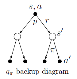
• 根据backup diagram写，先是一个\(p(s^\prime,r|s,a)\)转移到\(s^\prime\)，得到\(r\)。然后根据\(\pi\)选择动作\(a^\prime\)，得到\(G_{t+1}\)，即\(q_\pi(s^\prime,a^\prime)\)：

\[\begin{array}{l} q_\pi(s,a) \overset{.}{=} E_\pi[G_t|S_t=s,A_t=a] \\ \qquad \quad \ = E_\pi[R_{t+1}+\gamma G_{t+1}|S_t=s,A_t=a] \\ \qquad \quad \ = \sum_{s^\prime,r}p(s^\prime,r|s,a)[r+\gamma \sum_{a^\prime}\pi(a^\prime|s^\prime)E_\pi[G_{t+1}|S_{t+1}=s^\prime,A_{t+1}=a^\prime]] \\ \qquad \quad \ = \sum_{s^\prime,r}p(s^\prime,r|s,a)[r+\gamma \sum_{a^\prime}\pi(a^\prime|s^\prime)q_\pi(s^\prime,a^\prime)] \end{array} \]

3.18 The value of a state depends on the values of the actions possible in that state and on how likely each action is to be taken under the current policy. We can think of this in terms of a small backup diagram rooted at the state and considering each possible action:

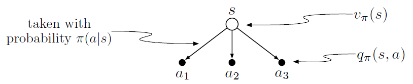
Give the equation corresponding to this intuition and diagram for the value at the root node, \(v_\pi(s)\), in terms of the value at the expected leaf node, \(q_\pi(s, a)\), given \(S_t = s\). This equation should include an expectation conditioned on following the policy, \(\pi\). Then give a second equation in which the expected value is written out explicitly in terms of \(\pi(a|s)\) such that no expected value notation appears in the equation.

• 这段话说的很清楚了，先写成\(q_\pi(s, a)\)的期望，再展开成\(\pi(a|s)\)的形式：

\[\begin{array}{l} v_\pi(s)=E_{a\sim\pi}[q_\pi(s,a)] \\ \qquad \ \ = \sum_a \pi(a|s)q_\pi(s,a) \end{array} \]

3.19
The value of an action, \(q_\pi(s, a)\), depends on the expected next reward and the expected sum of the remaining rewards. Again we can think of this in terms of a small backup diagram, this one rooted at an action (state–action pair) and branching to the possible next states:

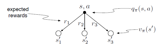
Give the equation corresponding to this intuition and diagram for the action value, \(q_\pi(s, a)\), in terms of the expected next reward, \(R_{t+1}\), and the expected next state value, \(v_\pi(S_{t+1})\), given that \(S_t=s\) and \(A_t=a\). This equation should include an expectation but not one conditioned on following the policy. Then give a second equation, writing out the expected value explicitly in terms of \(p(s^\prime, r|s, a)\) defined by (3.2), such that no expected value notation appears in the equation.

• 同上题：

\[\begin{array}{l} q_\pi(s,a)=E[R_{t+1}+\gamma v_\pi(s^\prime)|S_t=s,A_t=a] \\ \qquad \ \ = \sum_{s^\prime,r} p(s^\prime,r|s,a)[r+\gamma v_\pi(s^\prime)] \end{array} \]

• 这里期望里面的\(G_{t+1}\)变成了\(v_\pi\)，里面的项已经和\(\pi\)无关了，所以外面的期望没有\(\pi\)的期望项了，只有关于\(s^\prime,r\)的。

3.20
Draw or describe the optimal state-value function for the golf example.

• 这里主要是知道高尔夫的例子在说啥，底层人民没玩过，看了半天。大概意思是说一共有两个动作，putter和driver。putter是小幅度的推杆，走得近但是准确。driver是大幅度挥杆，打的远但是不够准。目标当然是打到洞里。最优决策是green外面用driver，里面用putter。整个图green外面同Figure 3.3 \(q_\star(s,driver)\)部分，green里面同\(v_{putt}\)部分。

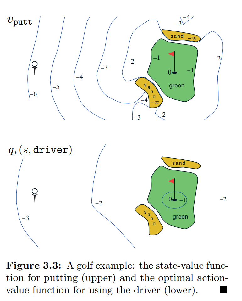
3.21 Draw or describe the contours of the optimal action-value function for putting, \(q_\star(s, putter)\), for the golf example.

• Figure 3.3 画的是\(q_\star(s,driver)\)，也就是第一步是driver，后面是最优决策的\(q\)值。现在让我们画\(q_\star(s, putter)\)，也就是第一步是putter，，后面是最优决策的\(q\)值。对比\(v_{putt}\)和\(q_\star(s,driver)\)的等高线，以图\(v_{putt}\)来说明位置。在-6的位置做putter，只能到-5的位置，还需要两次driver，再加一次putter，所以-6位置的值为-4。-5的位置做putter，到-4的位置，这个时候一次driver到green，再一次putter进洞，所以-5的位置为-3。剩下的同理。sand的地方要注意一下，一次putter还是在sand，然后driver一次到green，再一次putter进洞，所以是-3。最后得到位置和值的对应关系

state	\(q_\star(s,putter)\)
-6	-4
-5	-3
-4	-3
-3	-2
-2	-2
green	-1
sand	-3

3.22 Consider the continuing MDP shown on to the right. The only decision to be made is that in the top state, where two actions are available, left and right. The numbers show the rewards that are received deterministically after each action. There are exactly two deterministic policies, left and right. What policy is optimal if \(\gamma = 0\)? If \(\gamma = 0.9\)? If \(\gamma = 0.5\)?

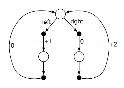
• 这个题搞了一个比较奇特的MDP，只能在最上面的状态做决策，而在下面两个状态没法做决策，但是reward还是要分别计算到两个状态上。所以有

\[v_{\pi_{left}}=1+\gamma\times0+\gamma^2\times 1+\gamma^3\times 0 +\gamma^4\times1 \cdots=\sum_{k=0}^\infty\gamma^{2k} \]

\[v_{\pi_{right}}=0+\gamma\times2+\gamma^2\times0+\gamma^3\times 2 +\gamma^4\times0 \cdots=2\sum_{k=0}^\infty\gamma^{2k+1} \]

所以有

\[\begin{array}{l} \gamma = 0 \rightarrow v_{\pi_{left}}=1 > v_{\pi_{right}}=0 \\ \gamma = 0.9 \rightarrow v_{\pi_{left}}\approx5.26 < v_{\pi_{right}}\approx 9.47 \\ \gamma = 0.5 \rightarrow v_{\pi_{left}}\approx1.33 = v_{\pi_{right}}\approx 1.33 \end{array} \]

3.23
Give the Bellman equation for \(q_*\) for the recycling robot.

• 给出\(q\)的贝尔曼最优方程，(3.20)：

\[q_*(s,a) = \sum_{r^\prime,s}p(s^\prime,r|s,a)[r+\gamma\max_{a^\prime}q_*(s^\prime,a^\prime)] \]

再根据Excercise(3.4)的表：

\(s\)	\(a\)	\(s^\prime\)	\(r\)	\(p(s^\prime,r|s,a)\)
high	search	high	\(r_{search}\)	\(\alpha\)
high	search	low	\(r_{search}\)	\(1-\alpha\)
high	wait	high	\(r_{wait}\)	1
low	wait	low	\(r_{wait}\)	1
low	recharge	high	0	1
low	search	high	-3	\(1-\beta\)
low	search	low	\(r_{search}\)	\(\beta\)

带入式子得到方程组：

\[\begin{array}{l} q_*(\text{high},\text{search}) = p(\text{high},r_{\text{search}}|\text{high},\text{search})[r_{\text{search}}+\gamma\max_{a^\prime}q_*(\text{high},a^\prime)] + \\ \qquad \qquad \qquad \qquad \ \ p(\text{low},r_{\text{search}}|\text{high},\text{search})[r_{\text{search}}+\gamma\max_{a^\prime}q_*(\text{low},a^\prime)] \\ q_*(\text{high},\text{wait}) = p(\text{high},r_{\text{wait}}|\text{high},\text{wait})[r_{\text{wait}}+\gamma\max_{a^\prime}q_*(\text{high},a^\prime)] \\ q_*(\text{low},\text{wait}) = p(\text{low},r_{\text{wait}}|low,\text{wait})[r_{\text{wait}}+\gamma\max_{a^\prime}q_*(\text{low},a^\prime)] \\ q_*(\text{low},\text{recharge}) = p(\text{high},0|\text{low},\text{recharge})[0+\gamma\max_{a^\prime}q_*(\text{high},a^\prime)] \\ q_*(\text{low},\text{search}) = p(\text{high},-3|\text{low},\text{search})[-3 + \gamma\max_{a^\prime}q_*(\text{high},a^\prime)] + \\ \qquad \qquad \qquad \qquad p(\text{low},r_{\text{search}}|\text{low},\text{search})[r_{\text{search}}+\gamma\max_{a^\prime}q_*(\text{low},a^\prime)] \end{array} \]

化简有：

\[\begin{array}{l} q_*(\text{high},\text{search}) = \alpha[r_{\text{search}}+\gamma\max_{a^\prime}q_*(\text{high},a^\prime)] + (1-\alpha)[r_{\text{search}}+\gamma\max_{a^\prime}q_*(\text{low},a^\prime)] \\ q_*(\text{high},\text{wait}) = r_{\text{wait}}+\gamma\max_{a^\prime}q_*(\text{high},a^\prime) \\ q_*(\text{low},\text{wait}) = r_{\text{wait}}+\gamma\max_{a^\prime}q_*(\text{low},a^\prime) \\ q_*(\text{low},\text{recharge}) = \gamma\max_{a^\prime}q_*(\text{high},a^\prime) \\ q_*(\text{low},\text{search}) = (1-\beta)[-3 + \gamma\max_{a^\prime}q_*(\text{high},a^\prime)] + \beta[r_{\text{search}}+\gamma\max_{a^\prime}q_*(\text{low},a^\prime)] \end{array} \]

3.24
Figure 3.5 gives the optimal value of the best state of the gridworld as 24.4, to one decimal place. Use your knowledge of the optimal policy and (3.8) to express this value symbolically, and then to compute it to three decimal places.

• 在24.4的位置刚好在\(\text{A}\)，这个位置的最优策略是先随便做一个动作，得到奖励值10，跳到\(\text{A}^\prime\)，然后一直往上走到\(\text{A}\)，中间得到奖励0。一直重复这个过程。直接根据(3.8)写：

\[\begin{array}{l} G_t \overset{.}{=} R_{t+1} + \gamma R_{t+2} + \gamma^2R_{t+3} + \cdots \\ \quad \ \ = 10 + \gamma^5\times10 + \gamma^{10}\times10 + \cdots \\ \quad \ \ = \frac{10}{1-0.9^5} \approx 24.419 \end{array} \]

3.25
Give an equation for \(v_*\)in terms of \(q_*\).

• 这个题公式(3.19)给的不是吗？还是我理解错了？

\[v_*(s)=\max_{a \in \mathcal{A}(s)}q_{\pi_*}(s,a) \]

3.26
Give an equation for \(q_*\) in terms of \(v_*\) and the four-argument \(p\).

• 接着公式(3.20)写：

\[q_*(s,a) = \sum_{s^\prime,r}p(s^\prime,r|s,a)[r+\gamma\max_{a^\prime}q_*(s^\prime,a^\prime)] = \sum_{s^\prime,r}p(s^\prime,r|s,a)[r+\gamma v_*(s^\prime)] \]

3.27 Give an equation for \(\pi_*\) in terms of \(q_*\).

• 这个不就是argmax吗，还是我没get到点？

\[\pi^*(a|s)= \left\{\begin{array}{l} 1,if \quad a=\arg\max\limits_{a \in A}q_*(s,a)\\ 0,otherwise \end{array}\right. \]

3.28 Give an equation for \(\pi_*\) in terms of \(v_*\) and the four-argument \(p\).

• 由3.26有：

\[q_*(s,a) = \sum_{s^\prime,r}p(s^\prime,r|s,a)[r+\gamma v_*(s^\prime)] \]

• 直接放到3.27中？

\[\pi^*(a|s)= \left\{\begin{array}{l} 1,if \quad a=\arg\max\limits_{a \in A}\sum_{s^\prime,r}p(s^\prime,r|s,a)[r+\gamma v_*(s^\prime)]\\ 0,otherwise \end{array}\right. \]

3.29 Rewrite the four Bellman equations for the four value functions \((v_\pi,v_*,q_\pi,and \ q_*)\) in terms of the three argument function \(p\) (3.4) and the two-argument function \(r\) (3.5).

• 先全列出来：

\[p(s^\prime|s,a) = \sum_{r \in \mathcal{R}}p(s^\prime,r|s,a) \]

\[r(s,a) = \sum_{r \in \mathcal{R}}r\sum_{s^\prime \in \mathcal{R}} p(s^\prime,r|s,a) \]

• 依次替换：

\[\begin{array}{l} v_\pi = \sum_a \pi(a|s)\sum_{s^\prime,r}p(s^\prime,r|s,a)[r+\gamma v_\pi(s^\prime)] \\ \quad \ =\sum_a \pi(a|s)[\sum_{r}\sum_{s^\prime}p(s^\prime,r|s,a)r+\sum_{s^\prime}\sum_{r}p(s^\prime,r|s,a)\gamma v_\pi(s^\prime)] \\ \quad \ =\sum_a \pi(a|s)[r(s,a)+\sum_{s^\prime}p(s^\prime|s,a)\gamma v_\pi(s^\prime)] \end{array} \]

\[\begin{array}{l} v_* = \max_{a}\sum_{s^\prime,r}p(s^\prime,r|s,a)[r+\gamma v_*(s^\prime)] \\ \quad \ =\max_{a}[\sum_{r}\sum_{s^\prime}p(s^\prime,r|s,a)r+\sum_{s^\prime}\sum_{r}p(s^\prime,r|s,a)\gamma v_*(s^\prime)] \\ \quad \ =\max_a[r(s,a)+\sum_{s^\prime}p(s^\prime|s,a)\gamma v_*(s^\prime)] \end{array} \]

\[\begin{array}{l} q_\pi(s,a) = \sum_{s^\prime,r}p(s^\prime,r|s,a)[r+\gamma \sum_{a^\prime}\pi(a^\prime|s^\prime)q_\pi(s^\prime,a^\prime)] \\ \qquad \quad \ \ = \sum_{r}\sum_{s^\prime}p(s^\prime,r|s,a)r+\sum_{s^\prime}\sum_{r}p(s^\prime,r|s,a)\gamma \sum_{a^\prime}\pi(a^\prime|s^\prime)q_\pi(s^\prime,a^\prime) \\ \qquad \quad \ \ = r(s,a)+\sum_{s^\prime}p(s^\prime|s,a)\gamma \sum_{a^\prime}\pi(a^\prime|s^\prime)q_\pi(s^\prime,a^\prime) \end{array} \]

\[\begin{array}{l} q_*(s,a) = \sum_{s^\prime,r}p(s^\prime,r|s,a)[r+\gamma\max_{a^\prime}q_\pi(s^\prime,a^\prime)] \\ \qquad \quad \ = \sum_{r}\sum_{s^\prime}p(s^\prime,r|s,a)r+\sum_{s^\prime}\sum_{r}p(s^\prime,r|s,a)\gamma\max_{a^\prime}q_\pi(s^\prime,a^\prime) \\ \qquad \quad \ = r(s,a)+\sum_{s^\prime}p(s^\prime|s,a)\gamma\max_{a^\prime}q_\pi(s^\prime,a^\prime) \end{array} \]

---

Chapter 4

4.1
In Example 4.1, if \(\pi\) is the equiprobable random policy, what is \(q_\pi(11, \text{down})\)? What is \(q_\pi(7, \text{down})\)?

• Figure 4.1给出了\(v_\pi\)，直接算\(q\)即可：\(q_\pi(11, \text{down}) = E_{s^\prime,r}[r+\gamma v_\pi(s^\prime)]=-1+0=-1\)。\(q_\pi(7, \text{down}) = -1-14=-15\)。

4.2
In Example 4.1, suppose a new state 15 is added to the gridworld just below state 13, and its actions, left, up, right, and down, take the agent to states 12, 13, 14, and 15, respectively. Assume that the transitions from the original states are unchanged. What, then, is \(v_\pi(15)\) for the equiprobable random policy? Now suppose the dynamics of state 13 are also changed, such that action down from state 13 takes the agent to the new state 15. What is \(v_\pi(15)\) for the equiprobable random policy in this case?

• 如果其他值都不变，那直接带进去算就行。

\[\begin{array}{l} v_\pi(15)=\sum_a\pi(a|s)\sum_{s^\prime,r}p(s^\prime,r|s,a)[r+\gamma v_\pi(s^\prime)] \\ \qquad \quad = \frac{1}{4}(-1-22)+\frac{1}{4}(-1-20)+\frac{1}{4}(-1-14)+\frac{1}{4}(-1+v_\pi(15)) \\ \\ \Rightarrow v_\pi(15) \approx -20 \end{array} \]

• 如果state 13也会变，那么就是一个二元方程组：

\[\begin{array}{l} \Rightarrow \left\{\begin{array}{l} v_\pi(15) = \frac{1}{4}(-1-22)+\frac{1}{4}(-1+v_\pi(13))+\frac{1}{4}(-1-14)+\frac{1}{4}(-1+v_\pi(15)) \\ \\ v_\pi(13)= \frac{1}{4}(-1-22)+\frac{1}{4}(-1-20)+\frac{1}{4}(-1-14)+\frac{1}{4}(-1+v_\pi(15)) \end{array}\right. \\ \\ \Rightarrow \left\{\begin{array}{l} v_\pi(15) = \frac{1}{4}(-39+v_\pi(13)+v_\pi(15)) \\ \\ v_\pi(13)= \frac{1}{4}(-60+v_\pi(15)) \end{array}\right. \\ \\ \Rightarrow \left\{\begin{array}{l} v_\pi(15) \approx -19.6 \\ \\ v_\pi(13) \approx -19.9 \end{array}\right. \end{array} \]

4.3
What are the equations analogous to (4.3), (4.4), and (4.5) for the actionvalue function \(q_\pi\) and its successive approximation by a sequence of functions \(q_0, q_1, q_2,\cdots\)?

• 照着之前的写

\[q_\pi(s,a) = E_\pi[R_{t+1}+\gamma G_{t+1}|S_t=s,A_t=a] \\ \qquad \qquad \qquad \quad = \sum_{s^\prime,r}p(s^\prime,r|s,a)[r+\gamma\sum_{a^\prime}\pi(a^\prime|s^\prime) q_\pi(s^\prime,a^\prime)] \\ \Rightarrow q_{k+1}(s,a)=\sum_{s^\prime,r}p(s^\prime,r|s,a)[r+\gamma\sum_{a^\prime}\pi(a^\prime|s^\prime) q_k(s^\prime,a^\prime)] \]

4.4 The policy iteration algorithm on page 80 has a subtle bug in that it may never terminate if the policy continually switches between two or more policies that are equally good. This is ok for pedagogy, but not for actual use. Modify the pseudocode so that convergence is guaranteed.

• 他这里说如果有两个策略一样好，那这个迭代过程就停不下来了。可以将终止条件改为两次policy evaluation的比较，如果两次evaluation得到的值估计不再变化，就终止。

4.5
How would policy iteration be defined for action values? Give a complete algorithm for computing \(q_*\), analogous to that on page 80 for computing \(v_*\). Please pay special attention to this exercise, because the ideas involved will be used throughout the rest of the book.

• 感觉式子是一样的，还是根据\(q_\pi(s,\pi^\prime(s)) \geq v_\pi(s)\)。只是之前维护的是\(v\)，现在要维护\(q\)。由\(v_\pi(s)=\sum_a\pi(a|s)q_\pi(s,a)\)，计算的时候拆开计算即可。

• policy evaluation里面更新\(q\)，

\[q_{k+1}(s,a) \leftarrow \sum_{s^\prime,r}p(s^\prime,r|s,a)[r+\gamma\sum_{a^\prime}\pi(a^\prime|s^\prime) q_k(s^\prime,a^\prime)] \]

• policy improvement里面更新\(\pi\)，

\[\pi(s) \leftarrow \arg\max_a\sum_{s^\prime,r}p(s^\prime,r|s,a)[r+\gamma \max_{a^\prime}q_k(s^\prime,a^\prime)] \]

4.6
Suppose you are restricted to considering only policies that are \(\epsilon-soft\), meaning that the probability of selecting each action in each state, \(s\), is at least \(\epsilon/|\mathcal{A}(s)|\). Describe qualitatively the changes that would be required in each of the steps 3, 2, and 1, in that order, of the policy iteration algorithm for \(v_*\) on page 80.

• step 3需要修改动作选择

\[\pi(s) = \left\{\begin{array}{l} \arg\max_a\sum_{s^\prime,r}p(s^\prime,r|s,a)[r+\gamma V(s^\prime)] \quad \text{with probability} \ 1-\epsilon \\ \text{random action \quad with probability} \ \epsilon \end{array}\right. \]

• step 2更新把\(\epsilon\)导致的动作选择概率考虑进去

\[V(s) \leftarrow \sum_a\pi(a|s)\sum_{s^\prime,r}p(s^\prime,r|s,a)[r+\gamma V(s^\prime)] \]

• step 1不用变，多初始化一个\(\epsilon\)就行。

4.7 (programming) Write a program for policy iteration and re-solve Jack’s car rental problem with the following changes. One of Jack’s employees at the first location rides a bus home each night and lives near the second location. She is happy to shuttle one car to the second location for free. Each additional car still costs $2, as do all cars moved in the other direction. In addition, Jack has limited parking space at each location. If more than 10 cars are kept overnight at a location (after any moving of cars), then an additional cost of $4 must be incurred to use a second parking lot (independent of how many cars are kept there). These sorts of nonlinearities and arbitrary dynamics often occur in real problems and cannot easily be handled by optimization methods other than dynamic programming. To check your program, first replicate the results given for the original problem.

4.8
Why does the optimal policy for the gambler’s problem have such a curious form? In particular, for capital of 50 it bets it all on one flip, but for capital of 51 it does not. Why is this a good policy?

• 这个题确实很奇怪，如果不是写代码跑一跑，很难想得到长这样。这里说一点感觉上的东西。首先关于中间50的这个地方，取50。先反过来想，要想赢，至少要上100，那么在50这个位置，不管从哪个地方到最后上100，最后一步都会乘一个概率\(p_h\)，也就是最后一步的\(p_h\)都一样。如果刚好下注50，也就是这个下注50就是最后一步了，要么赢，要么输，这个时候的值估计就是\(p_h=0.4\)。接下来说明其他下注的方式小于这个就行。假如投注小于这个值，那么不管输赢，这一次都不可能超过100，还必须经过多次投注，直到最后一个动作，经过概率概率\(p_h\)超过100，但是中间这么多过程的概率乘积肯定都是小于等于1的，也就是说\(p_1p_2...p_tp_h \leq p_h\)，也就是其他一连串的动作，胜率都不如直接50，所以再这个地方最优策略就是50。然后说一下为啥51突然就变成1了。这个也很难看出来。有个知觉的方法是，押注1如果输了，就转到50，然后就和50一样了。如果赢了，那就变成了52了，接下来的序列至少有概率会赢，所以51这个地方的值估计至少比50处的大。至于是不是最优的，感觉想不出来了。貌似押注49也比50处的大，哪个好就不知道了，感觉貌似一样。

4.9
(programming) Implement value iteration for the gambler’s problem and solve it for \(p_h = 0.25\) and \(p_h = 0.55\). In programming, you may find it convenient to introduce two dummy states corresponding to termination with capital of 0 and 100, giving them values of 0 and 1 respectively. Show your results graphically, as in Figure 4.3. Are your results stable as \(\theta \rightarrow 0\)?

4.10
What is the analog of the value iteration update (4.10) for action values, \(q_{k+1}(s, a)\)?

• 根据Excercise 4.5，给\(q_{k+1}(s,a) \leftarrow \sum_{s^\prime,r}p(s^\prime,r|s,a)[r+\gamma\sum_{a^\prime}\pi(a^\prime|s^\prime) q_k(s^\prime,a^\prime)]\)的\(\pi\)改成\(\max\)：

\[q_{k+1}(s,a) \leftarrow \sum_{s^\prime,r}p(s^\prime,r|s,a)[r+\gamma \max_{a^\prime} q_k(s^\prime,a^\prime)] \]