
代码3-1 餐饮销量额数据缺失值及异常值检测代码
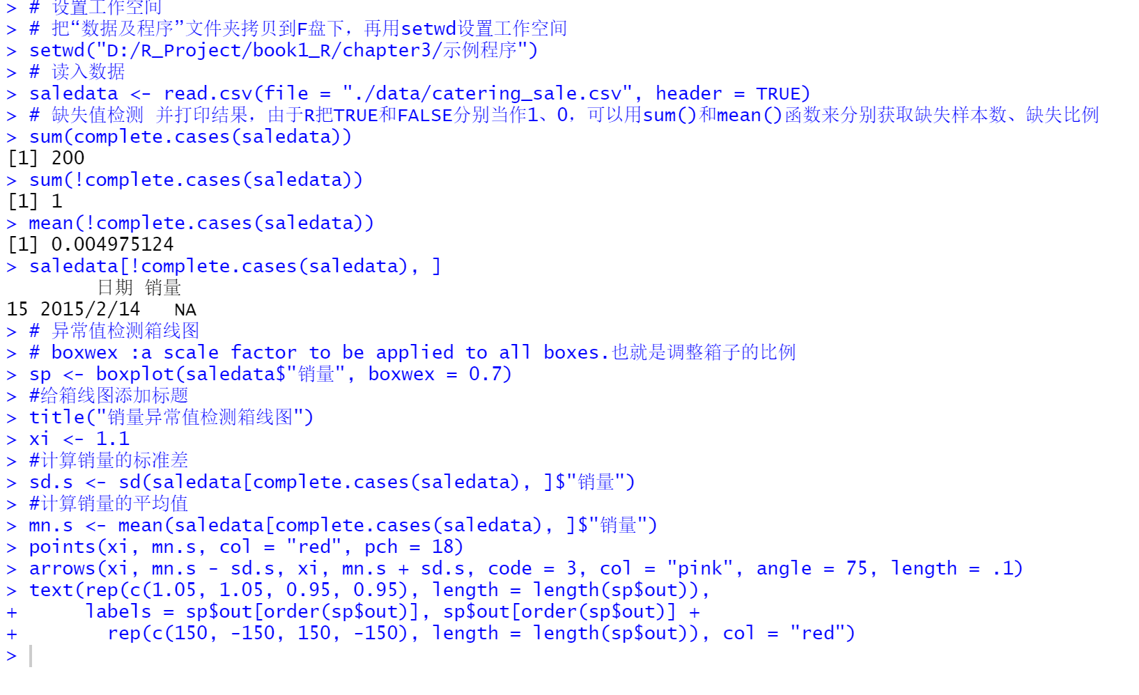
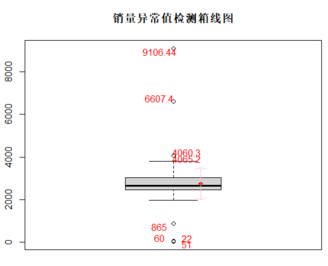
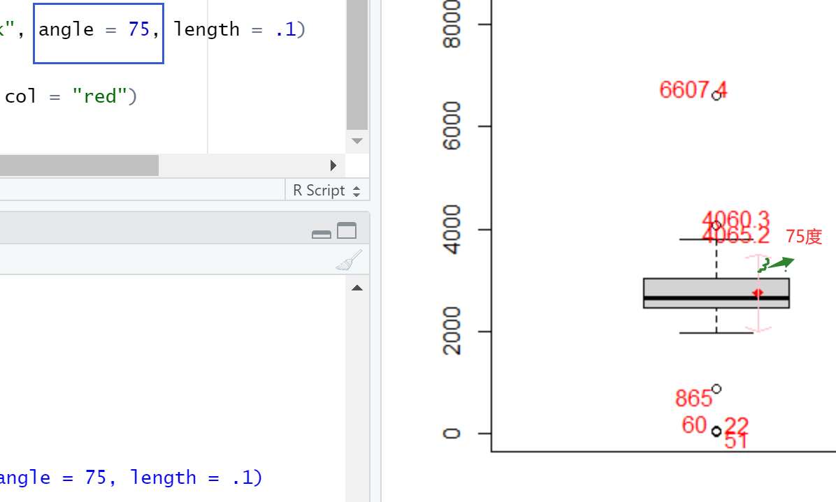
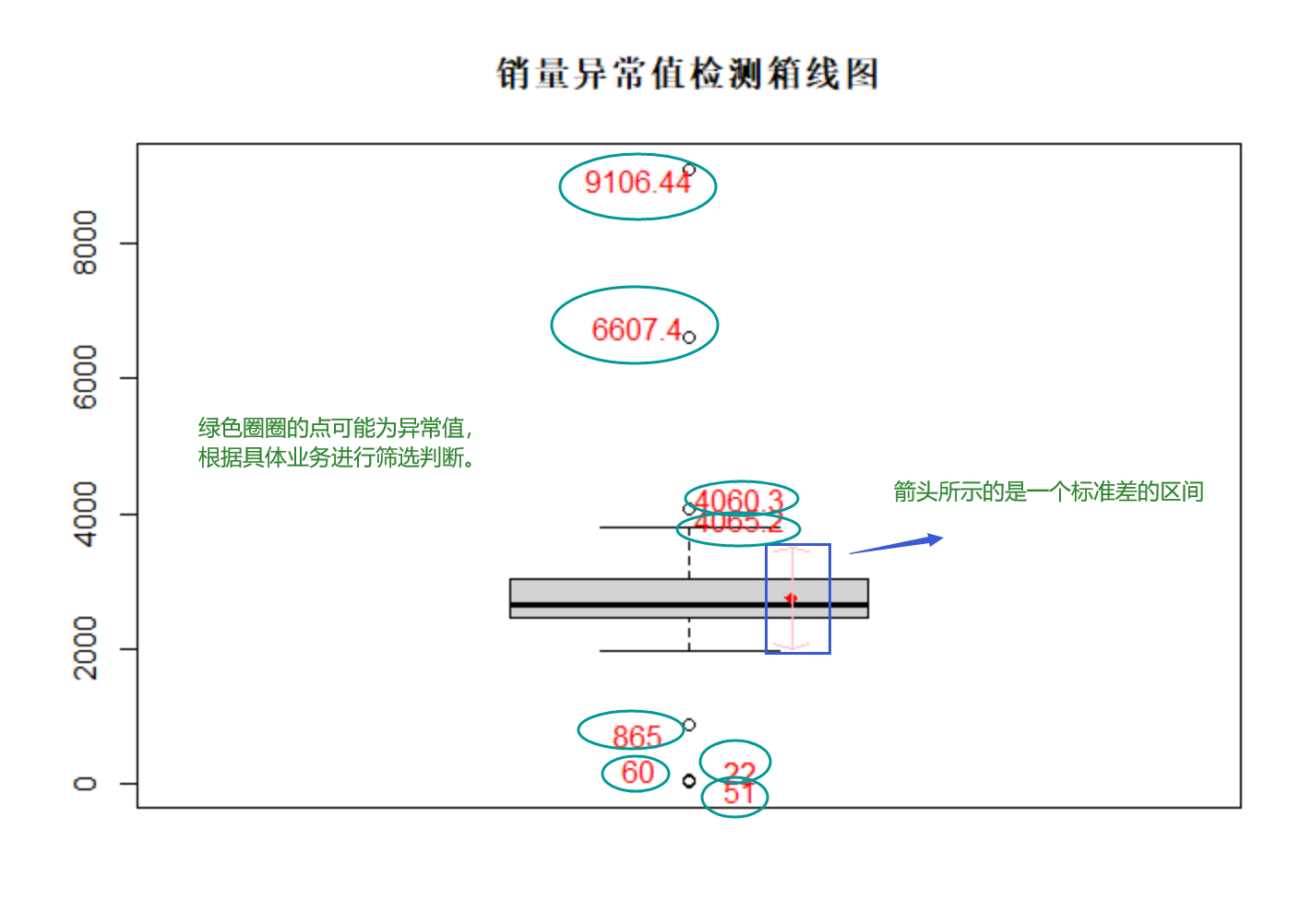
 1 # 设置工作空间
 2 # 把“数据及程序”文件夹拷贝到F盘下,再用setwd设置工作空间
 3 setwd("D:/R_Project/book1_R/chapter3/示例程序")
 4 # 读入数据
 5 saledata <- read.csv(file = "./data/catering_sale.csv", header = TRUE)
 6
 7 # 缺失值检测 并打印结果,由于R把TRUE和FALSE分别当作1、0,可以用sum()和mean()函数来分别获取缺失样本数、缺失比例
 8 sum(complete.cases(saledata))
 9 sum(!complete.cases(saledata))
10 mean(!complete.cases(saledata))
11 saledata[!complete.cases(saledata), ]
12
13 # 异常值检测箱线图
14 # boxwex :a scale factor to be applied to all boxes.也就是调整箱子的比例
15 sp <- boxplot(saledata$"销量", boxwex = 0.7)
16 #给箱线图添加标题
17 title("销量异常值检测箱线图")
18
19 xi <- 1.1
20
21 #计算销量的标准差
22 sd.s <- sd(saledata[complete.cases(saledata), ]$"销量")
23
24 #计算销量的平均值
25 mn.s <- mean(saledata[complete.cases(saledata), ]$"销量")
26 points(xi, mn.s, col = "red", pch = 18)
27 arrows(xi, mn.s - sd.s, xi, mn.s + sd.s, code = 3, col = "pink", angle = 75, length = .1)
28 text(rep(c(1.05, 1.05, 0.95, 0.95), length = length(sp$out)),
29      labels = sp$out[order(sp$out)], sp$out[order(sp$out)] +
30        rep(c(150, -150, 150, -150), length = length(sp$out)), col = "red")
Notes:
(1)

(2)
* R语言用complete.cases 和 na.omit去除有空值的行:http://blog.sina.com.cn/s/blog_59990a450101qnvy.html
* complete.cases()函数:Return a logical vector indicating which cases are complete, i.e., have no missing values.
* 也就是说它返回的是一个TRUE/FALSE的逻辑向量
(3)
* points()函数:用于标记某个点,设定参数pch即标记该点要用什么形状的来标记,pch=20是实心圆形状;设定参数cex表示这个形状的大小设定为多少,一般cex=2就够了;参数col设定点的颜色
* pch
* plotting ‘character’, i.e., symbol to use. This can either be a single character or an integer code for one of a set of graphics symbols.The full set of S symbols is available with pch = 0:18, see the examples below. (NB: R uses circles instead of the octagons used in S.) Value pch = "." (equivalently pch = 46) is handled specially. It is a rectangle of side 0.01 inch (scaled by cex). In addition, if cex = 1 (the default), each side is at least one pixel (1/72 inch on the pdf, postscript and xfig devices). For other text symbols, cex = 1 corresponds to the default fontsize of the device, often specified by an argument pointsize. For pch in 0:25 the default size is about 75% of the character height (see par("cin")).
* cex
* character (or symbol) expansion: a numerical vector. This works as a multiple of par("cex").
(4)
* arrows()函数:用于在图像画箭头的函数
* 定义:arrows(x0, y0, x1 = x0, y1 = y0, length = 0.25, angle = 30,code = 2, col = par("fg"), lty = par("lty"),lwd = par("lwd"), ...)
* Argument:
* x0, y0
* coordinates of points from which to draw.
* x1, y1
* coordinates of points to which to draw. At least one must the supplied
* length
* length of the edges of the arrow head (in inches).
* angle
* angle from the shaft of the arrow to the edge of the arrow head.(从箭头的轴到箭头的边缘的角度。)
* code
* integer code, determining kind of arrows to be drawn.
* col, lty, lwd
* graphical parameters, possible vectors. NA values in col cause the arrow to be omitted.
箱线图分析:
代码3-2 餐饮销量额数据缺失值及异常值检测代码
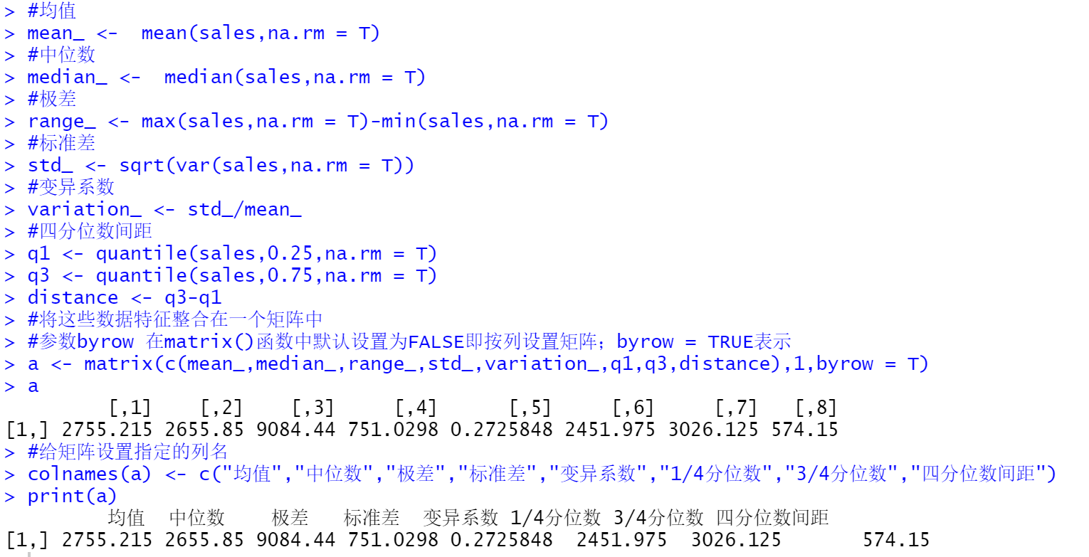
 1 #设置工作空间
 2 #把"数据及程序"文件夹复制到D盘下,再用setwd设置工作空间
 3 setwd("D:/R_Project/Practice_book1/")
 4
 5 #读入数据
 6 saledata = read.table(file = "./chapter03/catering_sale.csv",sep = ",",header = T)
 7
 8 sales = saledata[,2]
 9
10 #统计分析
11 #参数na.rm设置为TRUE,表示操作数据时,遇到NA不管
12
13 #均值
14 mean_ <-  mean(sales,na.rm = T)
15
16 #中位数
17 median_ <-  median(sales,na.rm = T)
18
19 #极差
20 range_ <- max(sales,na.rm = T)-min(sales,na.rm = T)
21
22 #标准差
23 std_ <- sqrt(var(sales,na.rm = T))
24
25 #变异系数
26 variation_ <- std_/mean_
27
28 #四分位数间距
29 q1 <- quantile(sales,0.25,na.rm = T)
30 q3 <- quantile(sales,0.75,na.rm = T)
31 distance <- q3-q1
32
33 #将这些数据特征整合在一个矩阵中
34 #参数byrow 在matrix()函数中默认设置为FALSE即按列设置矩阵;byrow = TRUE表示
35 a <- matrix(c(mean_,median_,range_,std_,variation_,q1,q3,distance),1,byrow = T)
36 #给矩阵设置指定的列名
37 colnames(a) <- c("均值","中位数","极差","标准差","变异系数","1/4分位数","3/4分位数","四分位数间距")
38
39 print(a)
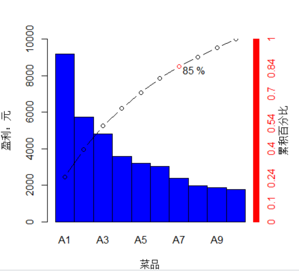
代码3-3 菜品盈利帕累图代码
 1 setwd("D:/R_Project/Practice_book1/chapter03/")
 2
 3 #读取菜品数据,绘制帕累托图
 4
 5 dishdata <- read.csv(file = "./catering_dish_profit.csv")
 6 barplot(dishdata[, 3], col = "blue1", names.arg = dishdata[, 2], width = 1,
 7         space = 0, ylim = c(0, 10000), xlab = "菜品", ylab = "盈利:元")
 8 accratio <- dishdata[, 3]
 9 for ( i in 1:length(accratio)) {
10   accratio[i] <- sum(dishdata[1:i, 3]) / sum(dishdata[, 3])
11 }
12
13 par(new = FALSE, mar = c(4, 4, 4, 4))
14 points(accratio * 10000 ~ c((1:length(accratio) - 0.5)), type = "b")
15 axis(4, col = "red", col.axis = "red", at = 0:10000, label = c(0:10000 / 10000))
16 mtext("累积百分比", 4, 2)
17
18 points(6.5, accratio[7] * 10000, col="red")
19 text(7.3, accratio[7] * 10000-200,paste(round(accratio[7] + 0.00001, 4) * 100, "%"))
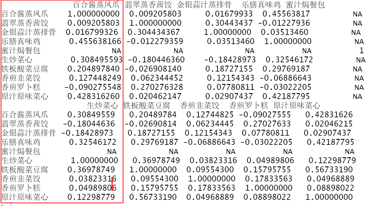
代码3-4 餐饮销量数据相关性分析
1 # 餐饮销量数据相关性分析
2 # 设置工作空间
3 # 把“数据及程序”文件夹拷贝到F盘下,再用setwd设置工作空间
4 setwd("D:/R_Project/book1_R/chapter3/示例程序")
5 # 读取数据
6 cordata <- read.csv(file = "./data/catering_sale_all.csv", header = TRUE)
7 # 求出相关系数矩阵
8 cor(cordata[, 2:11])
Notes:
|r|<=0.3 为极弱线性相关或不存在线性相关
0.3<|r|<=0.5 为低度线性相关
0.5<|r|<=0.8为显著线性相关
|r|>0.8 为高度线性相关
