
FRCN文本检测(转)
[源码分析]Text-Detection-with-FRCN
Text-Detection-with-FRCN项目是基于py-faster-rcnn项目在场景文字识别领域的扩展。对Text-Detection-with-FRCN的理解过程,本质上是对py-faster-rcnn的理解过程。我个人认为,初学者,尤其是对caffe还不熟悉的时候,在理解整个项目的过程中,会有以下困惑:
1.程序入口
2.数据是如何准备的?
3.整个网络是如何构建的?
4.整个网络是如何训练的?
那么,接下来,以我的理解,结合论文和源代码,一步步进行浅析。
一.程序入口
训练阶段:
入口一:/py-faster-rcnn/experiments/scripts/faster_rcnn_end2end.sh
-- >
入口二: /py-faster-rcnn/tools/train_net.py
在train_net中:
1.定义数据格式,获得imdb,roidb;
2.开始训练网络。
- train_net(args.solver, roidb, output_dir, pretrained_model, max_iters)
train_net定义在/py-faster-rcnn/lib/fast_rcnn/train.py中
-->
入口三:/py-faster-rcnn/lib/fast_rcnn/train.py
在train_net函数中:
- roidb = filter_roidb(roidb)
- sw = SolverWrapper(solver_prototxt, roidb, output_dir, pretrained_model=pretrained_model)
- model_paths = sw.train_model(max_iters)
- return model_paths
这样,就开始对整个网络进行训练了。
在solver_prototxt中,定义了train_prototxt。在train_prototxt中,定义了各种层,这些层组合起来,形成了训练网络的结构。
-->
入口四:/py-faster-rcnn/models/coco_text/VGG16/faster_rcnn_end2end/train.prototxt
先举例说明形式:
1.自定义Caffe Python layer
- layer {
- name: 'input-data'
- type: 'Python'
- top: 'data'
- top: 'im_info'
- top: 'gt_boxes'
- python_param {
- module: 'roi_data_layer.layer'
- layer: 'RoIDataLayer'
- param_str: "'num_classes': 2"
- }
- }
type为’python';
python_param中:
module为模块名,通常也是文件名。module: 'roi_data_layer.layer':说明这一层定义在roi_data文件夹下面的layer中
layer为模块里的类名。layer:'RoIDataLayer':说明该类的名字为'RoIDataLayer'
param_str为传入该层的参数。
2.caffe中原有的定义好的层,一般用c++定义。
- layer {
- name: "conv1_1"
- type: "Convolution"
- bottom: "data"
- top: "conv1_1"
- param {
- lr_mult: 0
- decay_mult: 0
- }
- param {
- lr_mult: 0
- decay_mult: 0
- }
- convolution_param {
- num_output: 64
- pad: 1
- kernel_size: 3
- }
- }
入口一: /py-faster-rcnn/tools/train_net.py
在train_net中:
获得imdb,roidb:imdb, roidb = combined_roidb(args.imdb_name)
进入位于 /py-faster-rcnn/tools/train_net.py,combined_roidb中:- def combined_roidb(imdb_names):
- def get_roidb(imdb_name):
- imdb = get_imdb(imdb_name)
- print 'Loaded dataset
{:s}for training'.format(imdb.name) - imdb.set_proposal_method(cfg.TRAIN.PROPOSAL_METHOD)
- print 'Set proposal method: {😒}'.format(cfg.TRAIN.PROPOSAL_METHOD)
- roidb = get_training_roidb(imdb)
- return roidb
- roidbs = [get_roidb(s) for s in imdb_names.split('+')]
- roidb = roidbs[0]
- if len(roidbs) > 1:
- for r in roidbs[1:]:
- roidb.extend(r)
- imdb = datasets.imdb.imdb(imdb_names)
- else:
- imdb = get_imdb(imdb_names)
- return imdb, roidb
先看imdb是如何产生的,然后看如何借助imdb产生roidb:
- def get_imdb(name):
- """Get an imdb (image database) by name."""
- if not __sets.has_key(name):
- raise KeyError('Unknown dataset: {}'.format(name))
- return __setsname
由此可见,get_imdb函数的实现原理:sets是一个字典,字典的key是数据集的名称,字典的value是一个lambda表达式(即一个函数指针)。
- case $DATASET in
- pascal_voc)
- TRAIN_IMDB="voc_2007_trainval"
- TEST_IMDB="voc_2007_test"
- PT_DIR="coco_text"
- ITERS=70000
- ;;
- # Set up voc<year><split> using selective search "fast" mode
- for year in ['2007', '2012']:
- for split in ['train', 'val', 'trainval', 'test']:
- name = 'voc{}{}'.format(year, split)
- _sets[name] = (lambda split=split, year=year: pascal_voc(split, year))
- class pascal_voc(imdb):
- def init(self, image_set, year, devkit_path=None):
- imdb.init(self, 'voc' + year + '' + image_set)
- self._year = year
- self._image_set = image_set
- # self._devkit_path = self._get_default_path() if devkit_path is None </span>
- # else devkit_path
- self._devkit_path = os.path.join(cfg.ROOT_DIR, '..', 'datasets', 'train_data')
- self._data_path = os.path.join(self._devkit_path, 'formatted_dataset')
- self._classes = ('background', # always index 0
- 'text')
- self._class_to_ind = dict(zip(self.classes, xrange(self.num_classes)))
- self._image_ext = '.jpg'
- self._image_index = self._load_image_set_index()
- # Default to roidb handler
- self._roidb_handler = self.selective_search_roidb
- self._salt = str(uuid.uuid4())
- self._comp_id = 'comp4'
- # PASCAL specific config options
- self.config = {'cleanup' : True,
- 'use_salt' : True,
- 'use_diff' : False,
- 'matlab_eval' : False,
- 'rpn_file' : None,
- 'min_size' : 2}
- assert os.path.exists(self._devkit_path),
- 'VOCdevkit path does not exist: {}'.format(self._devkit_path)
- assert os.path.exists(self.data_path),
- 'Path does not exist: {}'.format(self.data_path)
在pascal_voc的构造函数中,定义了imdb的结构,那么roidb与imdb有什么关系呢?
- imdb = get_imdb(imdb_name)
- print 'Loaded dataset
{:s}for training'.format(imdb.name) - imdb.set_proposal_method(cfg.TRAIN.PROPOSAL_METHOD)
- print 'Set proposal method: {😒}'.format(cfg.TRAIN.PROPOSAL_METHOD)
- roidb = get_training_roidb(imdb)
- return roidb
其中,set_proposal_method方法在/py-faster-rcnn/lib/datasets/imdb.py中:
- def set_proposal_method(self, method):
- method = eval('self.' + method + '_roidb')
- self.roidb_handler = method
所以set_proposal_method是用于设置生成proposal的方法。
- def get_training_roidb(imdb):
- """Returns a roidb (Region of Interest database) for use in training."""
- if cfg.TRAIN.USE_FLIPPED:
- print 'Appending horizontally-flipped training examples...'
- imdb.append_flipped_images()
- print 'done'
- print 'Preparing training data...'
- rdl_roidb.prepare_roidb(imdb)
- print 'done'
- return imdb.roidb
get_training_roidb方法中包含了两个方法:append_flipped_images() 和prepare_roidb()方法。
- def append_flipped_images(self):
- num_images = self.num_images
- widths = self._get_widths()
- for i in xrange(num_images):
- boxes = self.roidb[i]['boxes'].copy()
- oldx1 = boxes[:, 0].copy()
- oldx2 = boxes[:, 2].copy()
- boxes[:, 0] = widths[i] - oldx2 - 1
- boxes[:, 2] = widths[i] - oldx1 - 1
- assert (boxes[:, 2] >= boxes[:, 0]).all()
- entry = {'boxes' : boxes,
- 'gt_overlaps' : self.roidb[i]['gt_overlaps'],
- 'gt_classes' : self.roidb[i]['gt_classes'],
- 'flipped' : True}
- self.roidb.append(entry)
- self._image_index = self._image_index * 2
- def prepare_roidb(imdb):
- """Enrich the imdb's roidb by adding some derived quantities that
- are useful for training. This function precomputes the maximum
- overlap, taken over ground-truth boxes, between each ROI and
- each ground-truth box. The class with maximum overlap is also
- recorded.
- """
- sizes = [PIL.Image.open(imdb.image_path_at(i)).size
- for i in xrange(imdb.num_images)]
- roidb = imdb.roidb
- for i in xrange(len(imdb.image_index)):
- roidb[i]['image'] = imdb.image_path_at(i)
- roidb[i]['width'] = sizes[i][0]
- roidb[i]['height'] = sizes[i][1]
- # need gt_overlaps as a dense array for argmax
- gt_overlaps = roidb[i]['gt_overlaps'].toarray()
- # max overlap with gt over classes (columns)
- max_overlaps = gt_overlaps.max(axis=1)
- # gt class that had the max overlap
- max_classes = gt_overlaps.argmax(axis=1)
- roidb[i]['max_classes'] = max_classes
- roidb[i]['max_overlaps'] = max_overlaps
- # sanity checks
- # max overlap of 0 => class should be zero (background)
- zero_inds = np.where(max_overlaps 0)[0]
- assert all(max_classes[zero_inds] 0)
- # max overlap > 0 => class should not be zero (must be a fg class)
- nonzero_inds = np.where(max_overlaps > 0)[0]
- assert all(max_classes[nonzero_inds] != 0)
由此可见,roidb是imdb的一个成员变量,roidb是一个list(list的每个元素对应一张图片)。其中,list中的每个元素是一个字典,字典中存放的key包括:boxes, gt_overlaps, gt_classes, flipped, seg_areas, image, width, height, max_classes, max_overlaps。至此,就利用我们提供的数据集,准备好了roidb的相关信息。
- def _get_image_blob(roidb, scale_inds):
- """Builds an input blob from the images in the roidb at the specified
- scales.
- """
- num_images = len(roidb)
- processed_ims = []
- im_scales = []
- for i in xrange(num_images):
- im = cv2.imread(roidb[i]['image'])
- if roidb[i]['flipped']:
- im = im[:, ::-1, :]
- target_size = cfg.TRAIN.SCALES[scale_inds[i]]
- im, im_scale = prep_im_for_blob(im, cfg.PIXEL_MEANS, target_size,
- cfg.TRAIN.MAX_SIZE)
- im_scales.append(im_scale)
- processed_ims.append(im)
通过cv2.imread,实现了将图片读取到内存。
- # Get the input image blob, formatted for caffe
- im_blob, im_scales = _get_image_blob(roidb, random_scale_inds)
- blobs = {'data': im_blob}
- .....
- blobs['im_info'] = np.array(
- [[im_blob.shape[2], im_blob.shape[3], im_scales[0]]],
- dtype=np.float32)
也就是,对于一副任意大小的P×Q图像(假设P为短边,Q为长边),首先reshape到M×N,其中M由cfg.TRAIN.SCALES决定,N由cfg.TRAIN.MAX_SIZE决定。blob中的data为reshape后的图像。im_info=[M,N,scale_factor]则保存了此次缩放的所有信息。
- layer {
- name: "rpn_conv/3x3"
- type: "Convolution"
- bottom: "conv5_3"
- top: "rpn/output"
- param { lr_mult: 1.0 }
- param { lr_mult: 2.0 }
- convolution_param {
- num_output: 512
- kernel_size: 3 pad: 1 stride: 1
- weight_filler { type: "gaussian" std: 0.01 }
- bias_filler { type: "constant" value: 0 }
- }
- }
- layer {
- name: "rpn_cls_score"
- type: "Convolution"
- bottom: "rpn/output"
- top: "rpn_cls_score"
- param { lr_mult: 1.0 }
- param { lr_mult: 2.0 }
- convolution_param {
- num_output: 18 # 2(bg/fg) 9(anchors)
- kernel_size: 1 pad: 0 stride: 1
- weight_filler { type: "gaussian" std: 0.01 }
- bias_filler { type: "constant" value: 0 }
- }
- }
- layer {
- name: "rpn_bbox_pred"
- type: "Convolution"
- bottom: "rpn/output"
- top: "rpn_bbox_pred"
- param { lr_mult: 1.0 }
- param { lr_mult: 2.0 }
- convolution_param {
- num_output: 36 # 4 * 9(anchors)
- kernel_size: 1 pad: 0 stride: 1
- weight_filler { type: "gaussian" std: 0.01 }
- bias_filler { type: "constant" value: 0 }
- }
- }
- layer {
- name: 'rpn-data'
- type: 'Python'
- bottom: 'rpn_cls_score'
- bottom: 'gt_boxes'
- bottom: 'im_info'
- bottom: 'data'
- top: 'rpn_labels'
- top: 'rpn_bbox_targets'
- top: 'rpn_bbox_inside_weights'
- top: 'rpn_bbox_outside_weights'
- python_param {
- module: 'rpn.anchor_target_layer'
- layer: 'AnchorTargetLayer'
- param_str: "'feat_stride': 16"
- }
- }
- array([[ -83., -39., 100., 56.],
- [-175., -87., 192., 104.],
- [-359., -183., 376., 200.],
- [ -55., -55., 72., 72.],
- [-119., -119., 136., 136.],
- [-247., -247., 264., 264.],
- [ -35., -79., 52., 96.],
- [ -79., -167., 96., 184.],
- [-167., -343., 184., 360.]])
这个是rpn/output输出的feature map的(0,0)位置的anchor坐标。其中每行的4个值[x1,y1,x2,y2]代表矩阵左上角和右下角点的坐标。一共有9行,代表feature map中的每个点都会生成9个anchors。
- def generate_anchors(base_size=16, ratios=[0.5, 1, 2],
- scales=2np.arange(3, 6)):
- """
- Generate anchor (reference) windows by enumerating aspect ratios X
- scales wrt a reference (0, 0, 15, 15) window.
- """
- base_anchor = np.array([1, 1, base_size, base_size]) - 1
- ratio_anchors = _ratio_enum(base_anchor, ratios)
- anchors = np.vstack([_scale_enum(ratio_anchors[i, :], scales)
- for i in xrange(ratio_anchors.shape[0])])
- return anchors
- def _ratio_enum(anchor, ratios):
- """
- Enumerate a set of anchors for each aspect ratio wrt an anchor.
- """
- w, h, x_ctr, y_ctr = _whctrs(anchor)
- size = w h
- size_ratios = size / ratios
- ws = np.round(np.sqrt(size_ratios))
- hs = np.round(ws ratios)
- anchors = _mkanchors(ws, hs, x_ctr, y_ctr)
- return anchors
- def _scale_enum(anchor, scales):
- """
- Enumerate a set of anchors for each scale wrt an anchor.
- """
- w, h, x_ctr, y_ctr = _whctrs(anchor)
- ws = w scales
- hs = h scales
- anchors = _mkanchors(ws, hs, x_ctr, y_ctr)
- return anchors
- # 1. Generate proposals from bbox deltas and shifted anchors
- shift_x = np.arange(0, width) self._feat_stride
- shift_y = np.arange(0, height) self._feat_stride
- shift_x, shift_y = np.meshgrid(shift_x, shift_y)
- shifts = np.vstack((shift_x.ravel(), shift_y.ravel(),
- shift_x.ravel(), shift_y.ravel())).transpose()
b)累积得到anchors
- # add A anchors (1, A, 4) to
- # cell K shifts (K, 1, 4) to get
- # shift anchors (K, A, 4)
- # reshape to (KA, 4) shifted anchors
- A = self._num_anchors
- K = shifts.shape[0]
- all_anchors = (self._anchors.reshape((1, A, 4)) +
- shifts.reshape((1, K, 4)).transpose((1, 0, 2)))
- all_anchors = all_anchors.reshape((K A, 4))
- total_anchors = int(K A)
c)过滤掉不在原图内的anchors
- # only keep anchors inside the image
- inds_inside = np.where(
- (all_anchors[:, 0] >= -self._allowed_border) &
- (all_anchors[:, 1] >= -self._allowed_border) &
- (all_anchors[:, 2] < im_info[1] + self._allowed_border) & # width
- (all_anchors[:, 3] < im_info[0] + self._allowed_border) # height
- )[0]
- if not cfg.TRAIN.RPN_CLOBBER_POSITIVES:
- # assign bg labels first so that positive labels can clobber them
- labels[max_overlaps < cfg.TRAIN.RPN_NEGATIVE_OVERLAP] = 0
- # fg label: for each gt, anchor with highest overlap
- labels[gt_argmax_overlaps] = 1
- # fg label: above threshold IOU
- labels[max_overlaps >= cfg.TRAIN.RPN_POSITIVE_OVERLAP] = 1
- if cfg.TRAIN.RPN_CLOBBER_POSITIVES:
- # assign bg labels last so that negative labels can clobber positives
- labels[max_overlaps < cfg.TRAIN.RPN_NEGATIVE_OVERLAP] = 0
(2)筛选anchors
- # subsample positive labels if we have too many
- num_fg = int(cfg.TRAIN.RPN_FG_FRACTION * cfg.TRAIN.RPN_BATCHSIZE)
- fg_inds = np.where(labels 1)[0]
- if len(fg_inds) > num_fg:
- disable_inds = npr.choice(
- fg_inds, size=(len(fg_inds) - num_fg), replace=False)
- labels[disable_inds] = -1
- # subsample negative labels if we have too many
- num_bg = cfg.TRAIN.RPN_BATCHSIZE - np.sum(labels 1)
- bg_inds = np.where(labels == 0)[0]
- if len(bg_inds) > num_bg:
- disable_inds = npr.choice(
- bg_inds, size=(len(bg_inds) - num_bg), replace=False)
- labels[disable_inds] = -1
3.生成rpn_bbox_targets
- bbox_targets = np.zeros((len(inds_inside), 4), dtype=np.float32)
- bbox_targets = _compute_targets(anchors, gt_boxes[argmax_overlaps, :])
- def _compute_targets(ex_rois, gt_rois):
- """Compute bounding-box regression targets for an image."""
- assert ex_rois.shape[0] gt_rois.shape[0]
- assert ex_rois.shape[1] 4
- assert gt_rois.shape[1] == 5
- return bbox_transform(ex_rois, gt_rois[:, :4]).astype(np.float32, copy=False)
- def bbox_transform_inv(boxes, deltas):
- if boxes.shape[0] == 0:
- return np.zeros((0, deltas.shape[1]), dtype=deltas.dtype)
- boxes = boxes.astype(deltas.dtype, copy=False)
- widths = boxes[:, 2] - boxes[:, 0] + 1.0
- heights = boxes[:, 3] - boxes[:, 1] + 1.0
- ctr_x = boxes[:, 0] + 0.5 widths
- ctr_y = boxes[:, 1] + 0.5 heights
- dx = deltas[:, 0::4]
- dy = deltas[:, 1::4]
- dw = deltas[:, 2::4]
- dh = deltas[:, 3::4]
- pred_ctr_x = dx widths[:, np.newaxis] + ctr_x[:, np.newaxis]
- pred_ctr_y = dy heights[:, np.newaxis] + ctr_y[:, np.newaxis]
- pred_w = np.exp(dw) widths[:, np.newaxis]
- pred_h = np.exp(dh) heights[:, np.newaxis]
- pred_boxes = np.zeros(deltas.shape, dtype=deltas.dtype)
- # x1
- pred_boxes[:, 0::4] = pred_ctr_x - 0.5 pred_w
- # y1
- pred_boxes[:, 1::4] = pred_ctr_y - 0.5 pred_h
- # x2
- pred_boxes[:, 2::4] = pred_ctr_x + 0.5 pred_w
- # y2
- pred_boxes[:, 3::4] = pred_ctr_y + 0.5 pred_h
- return pred_boxes
- bbox_inside_weights = np.zeros((len(inds_inside), 4), dtype=np.float32)
- bbox_inside_weights[labels 1, :] = np.array(cfg.TRAIN.RPN_BBOX_INSIDE_WEIGHTS)
- bbox_outside_weights = np.zeros((len(inds_inside), 4), dtype=np.float32)
- if cfg.TRAIN.RPN_POSITIVE_WEIGHT < 0:
- # 实现均匀取样
- # uniform weighting of examples (given non-uniform sampling)
- num_examples = np.sum(labels >= 0)
- positive_weights = np.ones((1, 4)) 1.0 / num_examples
- negative_weights = np.ones((1, 4)) 1.0 / num_examples
- else:
- assert ((cfg.TRAIN.RPN_POSITIVE_WEIGHT > 0) &
- (cfg.TRAIN.RPN_POSITIVE_WEIGHT < 1))
- positive_weights = (cfg.TRAIN.RPN_POSITIVE_WEIGHT /
- np.sum(labels 1))
- negative_weights = ((1.0 - cfg.TRAIN.RPN_POSITIVE_WEIGHT) /
- np.sum(labels 0))
- bbox_outside_weights[labels 1, :] = positive_weights
- bbox_outside_weights[labels == 0, :] = negative_weights
- layer {
- name: "rpn_cls_score"
- type: "Convolution"
- bottom: "rpn/output"
- top: "rpn_cls_score"
- param { lr_mult: 1.0 }
- param { lr_mult: 2.0 }
- convolution_param {
- num_output: 18 # 2(bg/fg) * 9(anchors)
- kernel_size: 1 pad: 0 stride: 1
- weight_filler { type: "gaussian" std: 0.01 }
- bias_filler { type: "constant" value: 0 }
- }
- }
- layer {
- bottom: "rpn_cls_score"
- top: "rpn_cls_score_reshape"
- name: "rpn_cls_score_reshape"
- type: "Reshape"
- reshape_param { shape { dim: 0 dim: 2 dim: -1 dim: 0 } }
- }
- layer {
- name: "rpn_cls_prob"
- type: "Softmax"
- bottom: "rpn_cls_score_reshape"
- top: "rpn_cls_prob"
- }
- layer {
- name: 'rpn_cls_prob_reshape'
- type: 'Reshape'
- bottom: 'rpn_cls_prob'
- top: 'rpn_cls_prob_reshape'
- reshape_param { shape { dim: 0 dim: 18 dim: -1 dim: 0 } }
- }

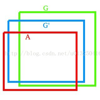
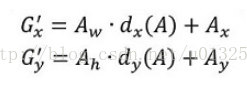
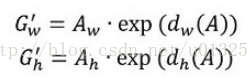
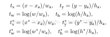
观察上面4个公式发现,需要学习的是dx(A),dy(A),dw(A),dh(A)这四个变换。当输入的anchor A与GT相差较小时,可以认为这种变换是一种线性变换, 那么就可以用线性回归来建模对窗口进行微调(注意,只有当anchors A和GT比较接近时,才能使用线性回归模型,否则就是复杂的非线性问题了)。对应于Faster RCNN原文,平移量(tx, ty)与尺度因子(tw, th)如下:

接下来的问题就是如何通过线性回归获得dx(A),dy(A),dw(A),dh(A)了。线性回归就是给定输入的特征向量X, 学习一组参数W, 使得经过线性回归后的值跟真实值Y非常接近,即Y=WX。对于该问题,输入X是一张经过卷积获得的feature map,定义为Φ;同时还有训练传入的GT,即(tx, ty, tw, th)。输出是dx(A),dy(A),dw(A),dh(A)四个变换。那么目标函数可以表示为:

其中Φ(A)是对应anchor的feature map组成的特征向量,w是需要学习的参数,d(A)是得到的预测值(表示 x,y,w,h,也就是每一个变换对应一个上述目标函数)。为了让预测值(tx, ty, tw, th)与真实值差距最小,设计损失函数:
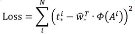
函数优化目标为:

- layer {
- name: "rpn_bbox_pred"
- type: "Convolution"
- bottom: "rpn/output"
- top: "rpn_bbox_pred"
- param { lr_mult: 1.0 }
- param { lr_mult: 2.0 }
- convolution_param {
- num_output: 36 # 4 9(anchors)
- kernel_size: 1 pad: 0 stride: 1
- weight_filler { type: "gaussian" std: 0.01 }
- bias_filler { type: "constant" value: 0 }
- }
- }
- layer {
- name: 'proposal'
- type: 'Python'
- bottom: 'rpn_cls_prob_reshape'
- bottom: 'rpn_bbox_pred'
- bottom: 'im_info'
- top: 'rpn_rois'
- # top: 'rpn_scores'
- python_param {
- module: 'rpn.proposal_layer'
- layer: 'ProposalLayer'
- param_str: "'feat_stride': 16"
- }
- }
- 生成anchors,利用[dx(A),dy(A),dw(A),dh(A)]对所有的anchors做bbox regression回归(这里的anchors生成和训练时完全一致)也就是说,前面的网络是对anchor进行训练,而proposal层是用来生成anchor。
- 按照输入的foreground softmax scores由大到小排序anchors,提取前pre_nms_topN(e.g. 6000)个anchors,即提取修正位置后的foreground anchors。
- 限定超出图像边界的foreground anchors为图像边界(防止后续roi pooling时proposal超出图像边界)
- 剔除非常小(width<threshold or height<threshold)的foreground anchors
- 进行nonmaximum suppression
- 再次按照nms后的foreground softmax scores由大到小排序fg anchors,提取前post_nms_topN(e.g. 300)结果作为proposal输出。
缩进RoI Pooling层则负责收集proposal,并计算出proposal feature maps,送入后续网络。从图2中可以看到Rol pooling层有2个输入:
- 原始的feature maps
- RPN输出的proposal boxes(大小各不相同)
1)为何需要RoI Pooling
先来看一个问题:对于传统的CNN(如AlexNet,VGG),当网络训练好后输入的图像尺寸必须是固定值,同时网络输出也是固定大小的vector or matrix。如果输入图像大小不定,这个问题就变得比较麻烦。有2种解决办法:
- 从图像中crop一部分传入网络
- 将图像warp成需要的大小后传入网络
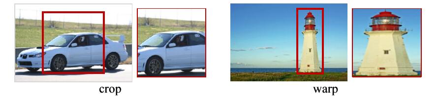
crop与warp破坏图像原有结构信息
两种办法的示意图如图,可以看到无论采取那种办法都不好,要么crop后破坏了图像的完整结构,要么warp破坏了图像原始形状信息。回忆RPN网络生成的proposals的方法:对foreground anchors进行bound box regression,那么这样获得的proposals也是大小形状各不相同,即也存在上述问题。所以Faster RCNN中提出了RoI Pooling解决这个问题。
2)RoI Pooling原理
缩进
分析之前先来看看RoI Pooling Layer的train.prototxt的定义:
- layer {
- name: "roi_pool5"
- type: "ROIPooling"
- bottom: "conv5_3"
- bottom: "rois"
- top: "pool5"
- roi_pooling_param {
- pooled_w: 7
- pooled_h: 7
- spatial_scale: 0.0625 # 1/16
- }
- }
其中有新参数pooled_w=pooled_h=7。
RoI Pooling layer forward过程:在之前有明确提到:proposal=[x1, y1, x2, y2]是对应MxN尺度的,所以首先使用spatial_scale参数将其映射回(M/16)x(N/16)大小的feature maps尺度;之后将每个proposal水平和竖直都分为7份,对每一份都进行max pooling处理。这样处理后,即使大小不同的proposal,输出结果都是7x7大小,实现了fixed-length output(固定长度输出)。
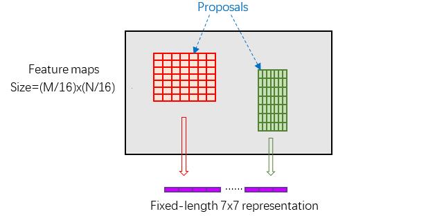
proposal示意图
- template <typename Dtype>
- void ROIPoolingLayer<Dtype>::Forward_cpu(const vector<Blob<Dtype>>& bottom,
- const vector<Blob<Dtype>>& top) {
- //conv5-3信息
- const Dtype bottom_data = bottom[0]->cpu_data();
- //rois信息
- const Dtype bottom_rois = bottom[1]->cpu_data();
- //Number of ROIs
- int num_rois = bottom[1]->num();
- //样本大小
- int batch_size = bottom[0]->num();
- int top_count = top[0]->count();
- //初始化top_data 和 argmax_data两个数组
- //caffe_set(const int N, const Dtype alpha, Dtype argmax_data);
- Dtype top_data = top[0]->mutable_cpu_data();
- caffe_set(top_count, Dtype(-FLT_MAX), top_data);
- int argmax_data = max_idx_.mutable_cpu_data();
- caffe_set(top_count, -1, argmax_data);
- // For each ROI R=[batch_index x1 y1 x2 y2]: max pool over R
- for (int n = 0; n < num_rois; ++n) {
- int roi_batch_ind = bottom_rois[0];
- //将生成的rois的坐标映射到原来的feature map上
- //rois中只包含了坐标信息,而不包含feature map信息
- int roi_start_w = round(bottom_rois[1] spatial_scale_);
- int roi_start_h = round(bottom_rois[2] spatial_scale_);
- int roi_end_w = round(bottom_rois[3] spatial_scale_);
- int roi_end_h = round(bottom_rois[4] spatial_scale_);
- CHECK_GE(roi_batch_ind, 0);
- CHECK_LT(roi_batch_ind, batch_size);
- //每一个region在feature map上对应的大小
- int roi_height = max(roi_end_h - roi_start_h + 1, 1);
- int roi_width = max(roi_end_w - roi_start_w + 1, 1);
- //每一个sub region的大小
- const Dtype bin_size_h = static_cast<Dtype>(roi_height) / static_cast<Dtype>(pooled_height_);
- const Dtype bin_size_w = static_cast<Dtype>(roi_width) / static_cast<Dtype>(pooled_width_);
- const Dtype batch_data = bottom_data + bottom[0]->offset(roi_batch_ind);
- for(int c = 0; c < channels_; ++c) {
- for(int ph = 0; ph < pooled_height_; ++ph) {
- for(int pw = 0; pw < pooled_width_; ++pw) {
- // Compute pooling region for this output unit:
- // start (included) = floor(ph roi_height / pooled_height__)
- // end (excluded) = ceil((ph+1) roi_height / pooled_height_)
- //floor(x):取小于等于x的整数,ceil(x):取大于x的整数
- //取得每一个sub region的起点终点坐标
- int hstart = static_cast<int>(floor(static_cast<DType>(ph) bin_size_h));
- int wstart = static_cast<int>(floor(static_cast<DType>(pw) bin_size_w));
- int hend = static_cast<int>(ceil(static_cast<DType>(ph+1) bin_size_h));
- int wend = static_cast<int>(ceil(static_cast<DType>(pw+1) bin_size_w));
- hstart = min(max(hstart + roi_start_h, 0), height_);
- hend = min(max(hend + roi_start_h, 0), height_);
- wstart = min(max(wstart + roi_start_w, 0), width_);
- wend = min(max(wend + roi_start_w, 0), width_);
- //剔除无效的roi
- bool is_empty = (hend <= hstart) || (wend <= wstart);
- //池化区域的编号
- const int pool_index = ph pooled_width_ + pw;
- if(is_empty){
- //如果该区域无效,则将池化结果设为0
- top_data[pool_index] = 0;
- //将最大区域的index设为-1
- argmax_data[pool_index] = -1;
- }
- //进行最大池化操作
- //pool_index:77的某一个池化区域的索引,index:feature map某一点的索引
- for(int h = hstart; h < hend; ++h) {
- for(int w = wstart; w < wend; ++w){
- //计算在feature map中的索引
- const int index = h width_ + w;
- if(batch_data[index] > top_data[pool_index]){
- top_data[pool_index] = batch_data[index];
- argmax_data[pool_index] = index;
- }
- }
- }
- }
- }
- //Increment all data pointers by one channel
- //也就是,将指针指向下一个channel
- batch_data += bottom[0]->offset(0,1);
- top_data += top[0]->offset(0,1);
- argmax_data += max_idx_.offset(0,1);
- }
- //Increment ROI data pointer
- bottom_rois += bottom[1]->offset(1);
- }
- }
roi_height:region proposal的高度
缩进Classification部分利用已经获得的proposal feature maps,通过full connect层与softmax计算每个proposal具体属于哪个类别,输出cls_prob概率向量;同时再次利用bounding box regression获得每个proposal的位置偏移量bbox_pred,用于回归更加精确的目标检测框。Classification部分网络结构如下图。

从RoI Pooling获取到7x7=49大小的proposal feature maps后,送入后续网络,可以看到做了如下2件事:
- 通过全连接和softmax对proposals进行分类;
- 再次对proposals进行bounding box regression,获取更高精度的rect box。
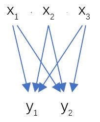
全连接层示意图
其计算公式如下:

其中W和bias B都是预先训练好的,即大小是固定的,当然输入X和输出Y也就是固定大小。所以,也就印证了Roi Pooling的必要性。
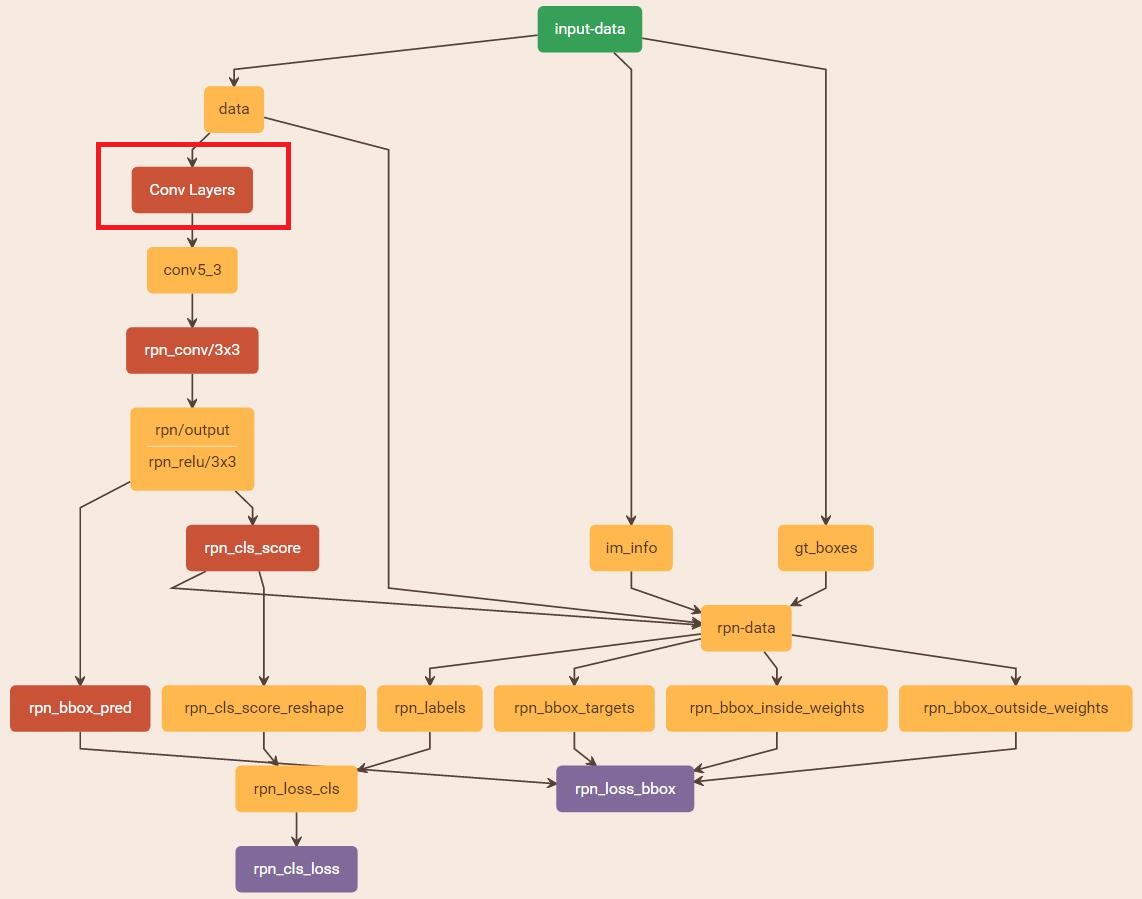
与检测网络类似的是,依然使用Conv Layers提取feature maps。整个网络使用的Loss如下:
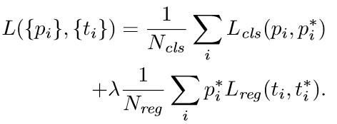
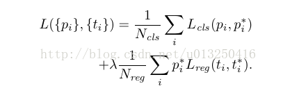
在上述公式中,i表示anchors index,pi表示foreground softmax predict概率,pi代表对应的GT predict概率(即当第i个anchor与GT间IoU>0.7,认为是该anchor是foreground,pi=1;反之IoU<0.3时,认为是该anchor是background,pi=0;至于那些0.3<IoU<0.7的anchor则不参与训练);t代表predict bounding box,t代表对应foreground anchor对应的GT box。可以看到,整个Loss分为2部分:
- cls loss,即rpn_cls_loss层计算的softmax loss,用于分类anchors为forground与background的网络训练
- reg loss,即rpn_loss_bbox层计算的soomth L1 loss,用于bounding box regression网络训练。注意在该loss中乘了pi,相当于只关心foreground anchors的回归。
由于在实际过程中,Ncls和Nreg差距过大,用参数λ平衡二者(如Ncls=256,Nreg=2400时设置λ=10),使总的网络Loss计算过程中能够均匀考虑2种Loss。这里比较重要是Lreg使用的soomth L1 loss,计算公式如下:


- 在RPN训练阶段,rpn-data(python AnchorTargetLayer)层会按照和test阶段Proposal层完全一样的方式生成Anchors用于训练
- 对于rpn_loss_cls,输入的rpn_cls_scors_reshape和rpn_labels分别对应p与p,Ncls参数隐含在p与p的caffe blob的大小中
- 对于rpn_loss_bbox,输入的rpn_bbox_pred和rpn_bbox_targets分别对应t于t,rpn_bbox_inside_weigths对应p*,rpn_bbox_outside_weights对应1/Nreg。
特别需要注意的是,在训练和检测阶段生成和存储anchors的顺序完全一样,这样训练结果才能被用于检测!
2)通过训练好的RPN网络收集proposals
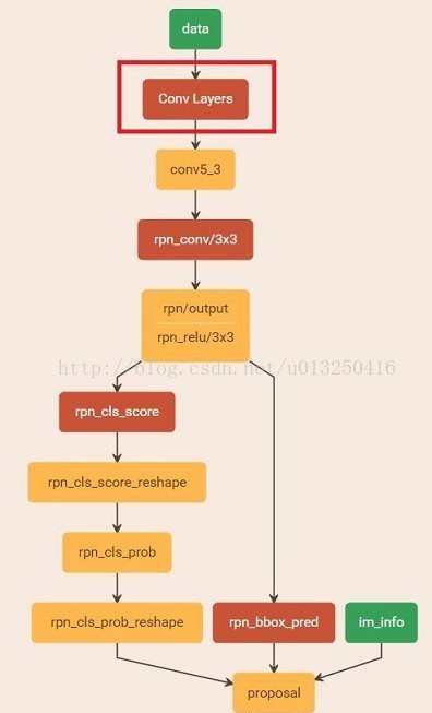
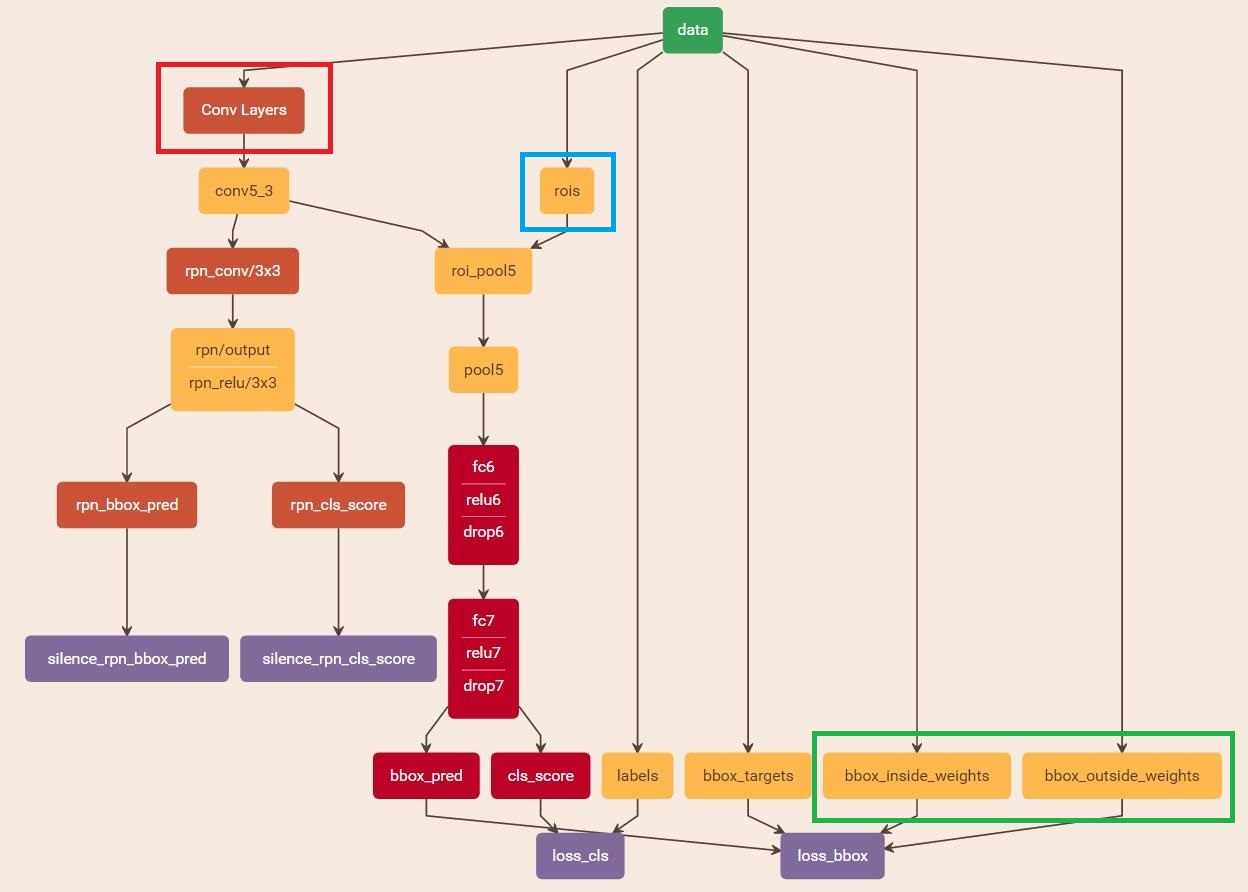
在该步骤中,利用之前的RPN网络,获取proposal rois,同时获取foreground softmax probability,如下图。注意:在前向传播中,将该部分看作是固定的,不对其计算loss。而实际上,本应该对proposal rois的坐标进行回归。所以,这种端到端的训练方式称为Approximate joint training。
如果是分步计算,此处应该产生loss。
- layer {
- name: 'proposal'
- type: 'Python'
- bottom: 'rpn_cls_prob_reshape'
- bottom: 'rpn_bbox_pred'
- bottom: 'im_info'
- top: 'rpn_rois'
- # top: 'rpn_scores'
- python_param {
- module: 'rpn.proposal_layer'
- layer: 'ProposalLayer'
- param_str: "'feat_stride': 16"
- }
- }
3)训练Faster RCNN网络
- layer {
- name: 'roi-data'
- type: 'Python'
- bottom: 'rpn_rois'
- bottom: 'gt_boxes'
- top: 'rois'
- top: 'labels'
- top: 'bbox_targets'
- top: 'bbox_inside_weights'
- top: 'bbox_outside_weights'
- python_param {
- module: 'rpn.proposal_target_layer'
- layer: 'ProposalTargetLayer'
- param_str: "'num_classes': 2"
- }
- }

 浙公网安备 33010602011771号