使用K-means和高斯混合模型对图像进行聚类

导入图片

?

1 2 3 4 5 6 7 8 9 10 11 12 13 14 15 16 17 18 19 20 21 22 23 24

%matplotlib inline import numpy as np  import skimage.io as SKimg  import matplotlib.pyplot as plt  from sklearn.cluster import KMeans from sklearn.mixture import GaussianMixture from skimage import io,data,color from scipy.ndimage import gaussian_filter from mpl_toolkits.mplot3d import Axes3D  # noqa: F401 unused import import time<br>import matplotlib.cm as cm   imgpath=r"H:\02Course\pics\35049.jpg" img =SKimg.imread(imgpath) io.imshow(img) print(type(img))  #显示类型 print(img.shape)  #显示尺寸 print('图片高度:',img.shape[0])  #图片高度 print('图片宽度:',img.shape[1])  #图片宽度 print('图片通道数:',img.shape[2])  #图片通道数 print('总像素个数:',img.size)   #显示总像素个数 print('最大像素值:',img.max())  #最大像素值 print('最小像素值:',img.min())  #最小像素值 print('像素平均值:',img.mean()) #像素平均值 print('图像的像素值:',img[0][0])#图像的像素值

?

1 2 3 4 5 6

image_height, image_width, image_channels = img.shape image_pixels = np.reshape(img, (-1, image_channels))#将三维矩阵转为通道特征矩阵  每列代表R G B值 _mean = np.mean(image_pixels,axis=0,keepdims=True) _std = np.std(image_pixels,axis=0,keepdims=True) image_pixels_ = (image_pixels - _mean) / _std # 归一化 X=image_pixels_ #特征矩阵

?

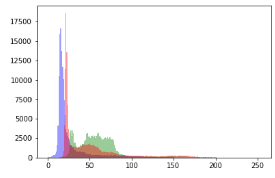
1 2 3

#绘制每个通道的直方图 Kwars=dict(histtype='stepfilled',alpha=0.4,bins=np.arange(0,255))#,normed=True intervals=plt.hist(image_pixels,color=[ "red","green","blue"],**Kwars)

 

?

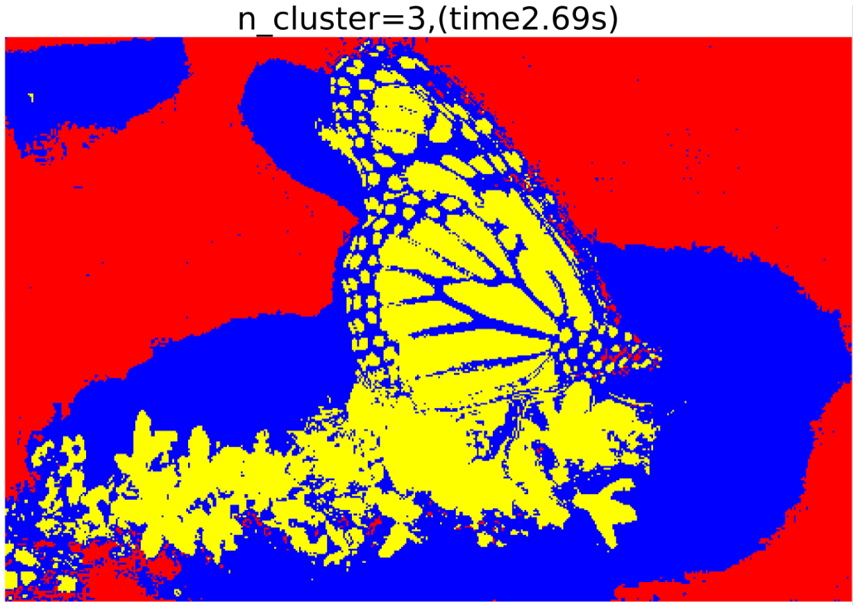
1 2 3 4 5 6 7 8 9 10 11 12 13 14 15 16 17 18 19 20 21 22 23 24 25 26 27 28 29 30 31 32 33 34 35 36 37 38 39 40 41 42 43 44 45 46 47 48 49 50 51 52 53 54 55 56 57 58 59 60 61 62 63

#聚类个数从3递增至8 for ncomp in range(3,9):     fig =plt.figure(figsize=(12,10))     plt.axis('off')     t0 = time.time()       gmm = GaussianMixture(n_components=ncomp,covariance_type='full').fit(X)#调用GMM算法，设置聚类的目标类别数     Clus_Centers=gmm.means_#每个类别的聚类中心     Labels=gmm.predict(X)       elapsed_time = time.time() - t0     Labels_show=np.reshape(Labels,(image_height, image_width))#把分类标签展开为二维数组     dst=color.label2rgb(Labels_show)#将标签转为RGB     plt.title('n_cluster=%i,(time%.2fs)'%(ncomp,elapsed_time), size=25)     plt.imshow(dst)     fig.savefig('pics/gmm_cluster_%i.jpg'%(ncomp), format='jpg', dpi=300,bbox_inches = 'tight',pad_inches = 0)#保存聚类结果图           Labels_arr=np.reshape(Labels_show, (-1, 1))     combine=np.append(image_pixels, Labels_arr, 1)     fig = plt.figure(figsize=(15, 10))     ax = plt.axes(projection='3d')     xs = combine[:,0]     ys = combine[:,1]     zs = combine[:,2]     ax.scatter(xs, ys, zs,c=combine[:,3],edgecolors='none',s=1)     ax.set_xlabel('R channel')     ax.set_ylabel('G channel')     ax.set_zlabel('B channel')     plt.show()     fig.savefig('pics/gmm_cluster3d_%i.jpg'%(ncomp), format='jpg', dpi=300,bbox_inches = 'tight',pad_inches = 0)#保存RGB通道三维特征空间图           fig = plt.figure(figsize=(6,5))     plt.xlabel('R channel')     plt.ylabel('G channel')     plt.axis('equal')     plt.xlim(0, 255)     plt.ylim(0, 255)     plt.scatter(combine[:, 0], combine[:, 1], c=combine[:,3],s=.2)     plt.colorbar()     plt.show()     fig.savefig('pics2/gmm_clusterR&G_%i.jpg'%(ncomp), format='jpg', dpi=300,bbox_inches = 'tight',pad_inches = 0)#保存RG通道二维特征空间图           fig = plt.figure(figsize=(6,5))     plt.xlabel('R channel')     plt.ylabel('B channel')     plt.axis('equal')     plt.xlim(0, 255)     plt.ylim(0, 255)     plt.scatter(combine[:, 0], combine[:, 2], c=combine[:,3],s=.2)     plt.colorbar()     plt.show()     fig.savefig('pics/gmm_clusterR&B_%i.jpg'%(ncomp), format='jpg', dpi=300,bbox_inches = 'tight',pad_inches = 0)#保存RB通道二维特征空间图           fig = plt.figure(figsize=(6,5))     plt.xlabel('G channel')     plt.ylabel('B channel')     plt.axis('equal')     plt.xlim(0, 255)     plt.ylim(0, 255)     plt.scatter(combine[:, 1], combine[:, 2], c=combine[:,3],s=.2)     plt.colorbar()     plt.show()     fig.savefig('pics/gmm_clusterG&B_%i.jpg'%(ncomp), format='jpg', dpi=300,bbox_inches = 'tight',pad_inches = 0)#保存GB通道二维特征空间图

 

聚类算法换位K-means，只需将聚类部分代码换为：

?

1 2	kmeans = KMeans(n_clusters=ncomp,random_state=0) Labels = kmeans.fit_predict(X)

　　

 

?

1 2 3 4 5 6 7 8

#高斯滤波 可平滑噪声 #替换即可 img =SKimg.imread(imgpath) img[:,:,0] = gaussian_filter(img[:,:,0], sigma=1) img[:,:,1] = gaussian_filter(img[:,:,1], sigma=1) img[:,:,2] = gaussian_filter(img[:,:,2], sigma=1) plt.axis('off') plt.imshow(img) plt.savefig('pics/gausfilter.jpg', format='jpg', dpi=300,bbox_inches = 'tight',pad_inches = 0)

　　

 

 

 

　　

　　

 

 

参考：

https://jakevdp.github.io/PythonDataScienceHandbook/05.12-gaussian-mixtures.html

https://scikit-learn.org/0.15/modules/generated/sklearn.mixture.GMM.html