CS231n笔记 Lecture 7, Training Neural Networks, Part 2

Review

Activation Functions. Sigmoid, tanh, ReLU(good default choice).

Optimization

• Optimization algorithms
  
  • SGD. Problems: jitering or stop at saddle point or local minima, noisy.
  • SGD + Momentum. Use velocity as a running mean of gradients, and use velocity instead of minibatch gradient to curve the noise and solve the problem of local minima and saddle points. Rho: gives "friction". Key Idea: Velocity, Curve sensitive.
    
  • Nesterov Momentum. $v_{t+1}=\rho v_t-\alpha\nabla f(x_t+\rho v_t)$, substitute variable to rearrange the equation, thus loss function and gradient will have the same input.
  • AdaGrad. Added element-wise scaling of the gradient based on the historical sum of squares in each dimension. On implementation, +eps in case of dividing by zero. Why AdaGrad: think about small gradient dimension and wiggling dimention. Good for convex optimization but bad when we have saddle points. Not commonly used for DNN cases.
  • RMSProp. Based on AdaGrad, solve the problem of smaller and smaller steps overtime. Key Idea: Making grad_squared decay.
  • Adam (Almost). maintain momentum(velocity) and scaling momentum(grad_squared) both (Momentum + AdaGrad/RMSProp), Problem: big first step.
  • Adam. plus bias correction. use an iteration count, and subtract the friction exponentially from 1 to make beginning steps small.
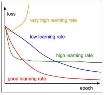
• pick a learning rate
  • Tricky trial: Adam, beta1 = 0.9, beta2 = 0.999, lr = 1e-3 or 5e-4
  • 

     

  • Learning rate decay. step decay, exponential decay $\alpha = \alpha_0e^{-kt}$. 1/t decay, $\alpha = \alpha_0 / (1 + kt)$. Common for SGD-momentum, less common for Adam.
  • lr decay is like a second order optimiztion, it will be very tricky, so start with no decay and see the loss map, then to decide whether to use decay or not.
• Second-Order Optimization
  
  • Impractical
• Model Ensembles
  • Train and Average multiple independent models
  • Polyak averaging

Regularization

• L2, L1, Elastic (combining L2 and L1)
• Dropout
  • Why make sense?
    • Forces the network to have a redundant representation;
    • Prevents co-adaptation of features
      or
    • Dropout is training a large ensemble of models (with shared parameters)
  • Dropout: Test time. At test time, to approximate the dropout behavior during the training time, we multiply the input (activation) of a nueron by the dropout probability.
    
  • More common: “Inverted dropout”. scale the activation during training so that at test time everything keeps unchanged.
Regularization strategy (common pattern) : randomness during training and average out randomness during test time.
• Example: BN
• Data Augmentation

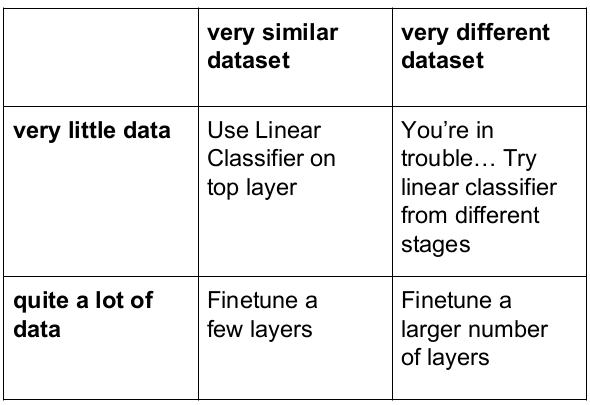
Transfer Learning

Don't train a nn from scratch, instead, use pretrained model as feature extractor, and