基于python的鸢尾花二分类

前言

也算是自己接触的第一个实例化的完整实现的小项目了吧（以前的的作业之类的都是没完全弄懂就交了不算哈），本此分享为简易鸢尾花的分类，实现语言是python 3.7，实现环境就是jupyter notebook。

1.数据集简介

本次数据集是从sklearn库中导入的load_iris()数据集，数据分四列，分别代表花萼长度、花萼宽度、花瓣长度、花瓣宽度，标签列或者说是target列有三种花种的类别数据表示分别是：'setosa', 'versicolor', 'virginica'；在数据集中以0，1，2 的形式展示。在本次实验中选择的是二分类任务这就要求我们对数据集进行一定的划分（这点的代码方面给了我很大的提升，个人觉得受益匪浅，我入坑的前进道路进了一大步）

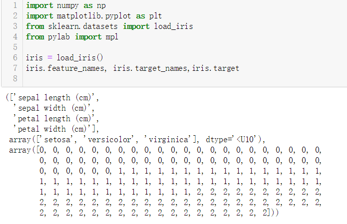
import numpy as np
import matplotlib.pyplot as plt
from sklearn.datasets import load_iris
from pylab import mpl

iris = load_iris()
iris.feature_names, iris.target_names,iris.target,iris,data  # 显示你需要看的所有数据

2.看看数据

下面我们来看看数据集的具体数字，如下图所示，四列是feature_names的数据，也就是花萼的有关数据，中间一行是target 也就是标签--花的种类，可以看到有50个0、50个1、50个2。

3.筛选数据并可视化

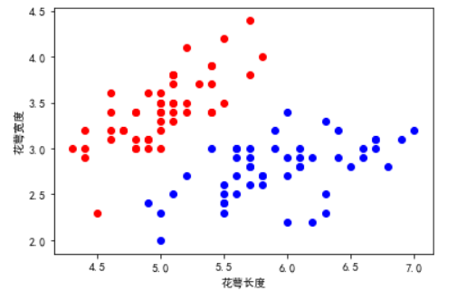
接下来就是数据筛选，我们选择二分类需要的数据，在这里决定对0和1进行分类，数据选择为前一百个。利用花萼长度和花萼宽度进行一个预测，四个数据的以此类推大致输出就是z = sigmoid（w1x1 + w2x2）,w是权重值，x是特征。

1 x = iris.data[0:100,0:2]  # 数据选择0到100行。前两列的标签数据，也就是0与1的花萼花瓣的数据
2 y = iris.target[0:100]    # 这是选中对应的前100个标签数据
3 samples_0 = x[y == 0,:]  # samples-0 是标签 y==0的集合
4 samples_1 = x[y == 1,:]  # samples-1 是标签 y==1的集合
5 plt.scatter(samples_0[:,0],samples_0[:,1],marker ='o',color = 'r')
6 plt.scatter(samples_1[:,0],samples_1[:,1],marker ='o',color = 'b')  #画出散点图
7 mpl.rcParams['font.sans-serif'] = ['SimHei']  # 没有这行代码，画出的图的xy轴标签数据会乱码没发现显示
8 plt.xlabel("花萼长度")
9 plt.ylabel("花萼宽度")

显示的图像如下：

接下来就是划分训练集和测试集;由于原始数据排列得很好所以我们要有预谋的进行打乱

xtrain = np.vstack([x[0:40,:],x[60:100,:]]) # 选中X的前40行和60到99行的数据，列数为X的所有列虽然只有2列
ytrain = np.concatenate([y[0:40],y[60:100]]) #把x对应的标签数据对应挑出来
xtest = x[40:60,:]  # 把剩下的当作数据集
ytest = y[40:60]   # 剩下的标签当作数据集
 
xtest.shape,ytest.shape

4.设计函数模型并输出

接下来就是定义Logistic类和各种函数了：

class LR():
    def __init__(self):
        self.w = None     # w就是我们要训练的权重值
        
    def sigmoid(self,z):
        a = 1/(1+ np.exp(-z))  # 也可以用lambda函数进行设置
        return a 
    
    def output(self,x):       # 输出嘛，肯定是经过sigmoid激活函数进行转换
        z = np.dot(self.w,x.T)
        a = self.sigmoid(z)
        return a 
    
    def comloss(self,x,y):
        numtrain = x.shape[0] # x 是数据 y是标签 输出的是x的行数，将0变成1就是列数
        a = self.output(x)
        loss = np.sum(-y * np.log(a) - (1-y)*np.log(1-a))/numtrain  # 自定义的损失函数，可以在这里进行调试
        dw = np.dot((a-y),x) / numtrain  # dot就是向量之间点乘的函数，dw是导数，这里用了梯度下降法
        
        return loss,dw
        
    def train(self,x,y,learningrate = 0.1,num_interations = 10000 ):   # 学习率就是梯度下降的直接影响步长的量，10000是迭代次数
        numtrain,numfeatures = x.shape
        self.w = 0.001 * np.random.randn(1,numfeatures)
        loss = []
        
        for i in range(num_interations):
            error,dw = self.comloss(x,y)
            loss.append(error)
            self.w -= learningrate * dw # 更新权重
            
            if i % 200 == 0:        # 每200次进行一次损失输出
                print('steps:[%d/%d],loss: %f' % (i,num_interations,error))
                
        return loss
    
    def predict(self,x):
        a = self.output(x)
        ypred = np.where(a >= 0.5,1,0)
        return ypred
    
LR = LR()
loss = LR.train(xtrain,ytrain)
plt.plot(loss)  


输出：
steps:[0/10000],loss: 0.692566
steps:[200/10000],loss: 0.237656
steps:[400/10000],loss: 0.155935
steps:[600/10000],loss: 0.121161
steps:[800/10000],loss: 0.101404
steps:[1000/10000],loss: 0.088442
steps:[1200/10000],loss: 0.079171
steps:[1400/10000],loss: 0.072148
steps:[1600/10000],loss: 0.066605
steps:[1800/10000],loss: 0.062095
steps:[2000/10000],loss: 0.058337
steps:[2200/10000],loss: 0.055146
steps:[2400/10000],loss: 0.052395
steps:[2600/10000],loss: 0.049991
steps:[2800/10000],loss: 0.047869
steps:[3000/10000],loss: 0.045979
steps:[3200/10000],loss: 0.044280
steps:[3400/10000],loss: 0.042744
steps:[3600/10000],loss: 0.041346
steps:[3800/10000],loss: 0.040068
steps:[4000/10000],loss: 0.038892
steps:[4200/10000],loss: 0.037806
steps:[4400/10000],loss: 0.036800
steps:[4600/10000],loss: 0.035864
steps:[4800/10000],loss: 0.034990
steps:[5000/10000],loss: 0.034173
steps:[5200/10000],loss: 0.033405
steps:[5400/10000],loss: 0.032683
steps:[5600/10000],loss: 0.032002
steps:[5800/10000],loss: 0.031358
steps:[6000/10000],loss: 0.030749
steps:[6200/10000],loss: 0.030170
steps:[6400/10000],loss: 0.029621
steps:[6600/10000],loss: 0.029097
steps:[6800/10000],loss: 0.028599
steps:[7000/10000],loss: 0.028122
steps:[7200/10000],loss: 0.027667
steps:[7400/10000],loss: 0.027231
steps:[7600/10000],loss: 0.026813
steps:[7800/10000],loss: 0.026413
steps:[8000/10000],loss: 0.026028
steps:[8200/10000],loss: 0.025657
steps:[8400/10000],loss: 0.025301
steps:[8600/10000],loss: 0.024958
steps:[8800/10000],loss: 0.024627
steps:[9000/10000],loss: 0.024308
steps:[9200/10000],loss: 0.023999
steps:[9400/10000],loss: 0.023701
steps:[9600/10000],loss: 0.023413
steps:[9800/10000],loss: 0.023134

损失表达图像：

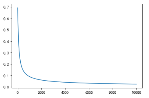
可以看出来经过梯度下降法的不断迭代其损失不断下降。

经过训练，权重值已经算出来了，接下来对其进行一个可视化;

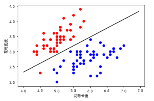
plt.scatter(samples_0[:,0],samples_0[:,1],marker ='o',color = 'r')
plt.scatter(samples_1[:,0],samples_1[:,1],marker ='o',color = 'b')
mpl.rcParams['font.sans-serif'] = ['SimHei']
plt.xlabel("花萼长度")
plt.ylabel("花萼宽度")
x1 = np.arange(4,7.5,0.05)   # 数据都是根据 数据集合理设置的 目的是为了不留太多空白
x2 = (-LR.w[0][0]* x1)/LR.w[0][1]  #
plt.plot(x1,x2,'-',color = 'black')

输出图像为;

为了便于读者理解，在这里加两行代码进行分析：

numtest = xtest.shape[0]
prediction = LR.predict(xtest)
acc = np.sum(prediction == ytest)/numtest
print("准确率",acc)
LR.w  # 输出最终预测的权重值


输出：

准确率 0.95

array([[  6.4110022 , -11.06167206]])

好了到此为止，预测，损失，训练的权重值，准确率都出来了，本次实验比较简单，但是折射出很多细节问题，还是值得小白入手训练的。

贴一下完整代码（其实上面就是完整了，为了减少学生白嫖党的烦恼还是总结一下吧，毕竟我也是这么过来的哈哈）：

import numpy as np
import matplotlib.pyplot as plt
from sklearn.datasets import load_iris
from pylab import mpl

iris = load_iris()
iris.feature_names, iris.target_names
x = iris.data[0:100,0:2]
y = iris.target[0:100]
samples_0 = x[y == 0,:]  # samples-0 是标签 y==0的集合
samples_1 = x[y == 1,:]  # samples-1 是标签 y==1的集合
plt.scatter(samples_0[:,0],samples_0[:,1],marker ='o',color = 'r')
plt.scatter(samples_1[:,0],samples_1[:,1],marker ='o',color = 'b')
mpl.rcParams['font.sans-serif'] = ['SimHei']
plt.xlabel("花萼长度")
plt.ylabel("花萼宽度")
# 划分数据集
xtrain = np.vstack([x[0:40,:],x[60:100,:]]) # 原始x 定义的是两列数据
ytrain = np.concatenate([y[0:40],y[60:100]]) #原始y 是标签值
xtest = x[40:60,:]
ytest = y[40:60]

xtest.shape,ytest.shape





class LR():
    def __init__(self):
        self.w = None
        
    def sigmoid(self,z):
        a = 1/(1+ np.exp(-z))
        return a 
    
    def output(self,x):
        z = np.dot(self.w,x.T)
        a = self.sigmoid(z)
        return a 
    
    def comloss(self,x,y):
        numtrain = x.shape[0] # x 是数据 y是标签 输出的是x的行数，1就是列数
        a = self.output(x)
        loss = np.sum(-y * np.log(a) - (1-y)*np.log(1-a))/numtrain
        dw = np.dot((a-y),x) / numtrain
        
        return loss,dw
        
    def train(self,x,y,learningrate = 0.1,num_interations = 10000 ):
        numtrain,numfeatures = x.shape
        self.w = 0.001 * np.random.randn(1,numfeatures)
        loss = []
        
        for i in range(num_interations):
            error,dw = self.comloss(x,y)
            loss.append(error)
            self.w -= learningrate * dw # 更新权重
            
            if i % 200 == 0:
                print('steps:[%d/%d],loss: %f' % (i,num_interations,error))
                
        return loss
    
    def predict(self,x):
        a = self.output(x)
        ypred = np.where(a >= 0.5,1,0)
        return ypred
    
LR = LR()
loss = LR.train(xtrain,ytrain)
plt.plot(loss)   




plt.scatter(samples_0[:,0],samples_0[:,1],marker ='o',color = 'r')
plt.scatter(samples_1[:,0],samples_1[:,1],marker ='o',color = 'b')
mpl.rcParams['font.sans-serif'] = ['SimHei']
plt.xlabel("花萼长度")
plt.ylabel("花萼宽度")
x1 = np.arange(4,7.5,0.05)
x2 = (-LR.w[0][0]* x1)/LR.w[0][1]
plt.plot(x1,x2,'-',color = 'black')



numtest = xtest.shape[0]
prediction = LR.predict(xtest)
acc = np.sum(prediction == ytest)/numtest
print("准确率",acc)
LR.w  # 输出最终预测的权重值

建议从上而下依次复现才会理解。

posted @ 2020-06-23 17:28 Anrys_Tian 阅读(4079) 评论(0) 编辑收藏举报

会员力量，点亮园子希望

刷新页面返回顶部

icetree

基于python的鸢尾花二分类

前言

公告