如下图所示,frenet坐标系下,给定边界,使用优化的思想求解轨迹
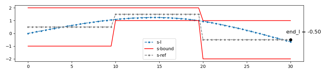
在frenet坐标系下,规划一条在平滑(舒适)、安全(限定空间)的轨迹。
定义代价函数包括平滑性、靠近中心线、终点,在上下边界内求解使代价函数最小的目标轨迹
Optimality Modeling
We consider the following factors in modeling the optimality of a path:
- Collision-free The path must not intersect with obstacles in the environment.
- Minimal lateral deviation If there is no collision risk, the vehicle should stay as close to the center of the lane as possible.
- Minimal lateral movement The lateral movement and its rate of change must be minimized. These two terms implicitly represent how quickly the vehicle moves laterally.
- (Optional)Maximal obstacle distance Maximize the distance between the vehicle and the obstacles to allow clearance for the vehicle to pass through safely. This factor turns out can be represented as the distance between the vehicle and the center of its corresponding path boundary.
从以下角度出发来规划和评价path:
1 无碰撞
2 最小横向偏差 - 沿中心线行驶
3 最小横向位移 - 降低横向位移和位移频率
4 (可选)远离障碍物
从而设计cost:
\[minimize\ f(l(s)) = w_l\cdot \int l(s)^2ds + w_{l'}\cdot \int l'(s)^2ds + w_{l''}\cdot \int l''(s)^2ds + w_{l'''}\cdot \int l'''(s)^2ds +\\
w_{obs} \cdot\int (l(s) - 0.5*(l_B(s)_{min} + l_B(s)_{max}))^2ds + \\
w_{end_l}\cdot (l_{n-1} - l_{endref})^2 + w_{end_{dl}}\cdot ({l}'_{n-1}-{l_{endref}}')^2 + w_{end_{ddl}}\cdot ({l}''_{n-1} - {l_{endref}}'')^2\\
\]
subject to the safety constraint:
\[l(s)\in l_B(s), \forall s\in [0,s_{max}]
\]
在cost中:
第一行表示平滑,l,l',l'',l'''最小
第二行表示中心线,尽量沿中心线行驶
第三行表示终点权重
To effectively formulate an optimization problem and evaluate constraint satisfaction in practice, our approach discretizes the path function l(s) according to the spatial parameter s to a certain resolution ∆s, and uses these discretized points to control the shape of the path, and approximately evaluate constraint satisfactions. Same ap- proach has been used in our previously published work . The key idea is to discretize the 1-dimensional function to second-order derivative level, and use constant third-order derivative terms to “connect” consecutive discretized points. Third order derivative of a positional variable is commonly named jerk. Thus this formulation is named piecewise-jerk method.
frenet坐标系下,沿固定距离△s将路径均匀采样
使用常三阶多项式连接各个点(每段曲线的三阶导数jerk为常量)
\[\begin{matrix} l_0\\l_0'\\l_0'' \end{matrix}
\overset{\Delta s}{\rightarrow}
\begin{matrix} l_1\\l_1'\\l_1'' \end{matrix}
\overset{\Delta s}{\rightarrow}
\begin{matrix} l_2\\l_2'\\l_2'' \end{matrix}
...
\begin{matrix} l_{n-2}\\l_{n-2}'\\l_{n-2}'' \end{matrix}
\overset{\Delta s}{\rightarrow}
\begin{matrix} l_{n-1}\\l_{n-1}'\\l_{n-1}'' \end{matrix}
\]
三阶导数是常量,那么有:
\[l_{i\rightarrow i+1}''' = \frac{l_{i+1}'' - l_i''}{\Delta s}
\]
积分得到:
\[{l_{i+1}}'' = \int_{0}^{\Delta s}{l_{i->i+1}}'''ds={l_i}''+{l_{i->i+1}}'''\cdot\Delta s\\
{l_{i+1}}'={l_i}'+\int_{0}^{\Delta s}{l}''(s)ds={l_i}'+{l_i}''\cdot\Delta s+\frac{1}{2}{l_{i->i+1}}'''\cdot\Delta s^2\\
l_{i+1}=l_i+\int_{0}^{\Delta s}{l}'(s)ds\\=l_i+(l_i)'\cdot\Delta s+\frac{1}{2}{l_i}''\cdot s^2+\frac{1}{6}{l_{i->i+1}}'''\cdot\Delta s^3
\]
qp problem
qp的一般形式
\[minimize \frac{1}{2} \cdot x^T \cdot P \cdot x + q \cdot x \\
s.t. LB \leq A\cdot x \leq UB
\]
将cost转为qp格式
以4个点P1,P2,P3,P4为例
我们要求解的矩阵x为:
\[\begin{vmatrix}
l_1\\
l_2\\
l_3\\
l_4\\
l_1'\\
l_2'\\
l_3'\\
l_4'\\
l_1''\\
l_2''\\
l_3''\\
l_4''\\
\end{vmatrix}
\]
先看cost中的平滑项:
\[w_l\cdot \sum_{i=0}^{n-1} l_i^2 + w_{{l}'}\cdot \sum_{i=0}^{n-1} {l_i}'^2 + w_{{l}''}\cdot \sum_{i=0}^{n-1} {l_i}''^2 + w_{{l}'''}\cdot \sum_{i=0}^{n-2}(\frac{{l_{i+1}}'' - {l_i}''}{\Delta s})^2 \\
\]
转为P矩阵
\[\begin{vmatrix}
w_l&0&0&0&0&0&0&0&0&0&0&0\\
0&w_l&0&0&0&0&0&0&0&0&0&0\\
0&0&w_l&0&0&0&0&0&0&0&0&0\\
0&0&0&w_l&0&0&0&0&0&0&0&0\\
0&0&0&0&w_{{l}'}&0&0&0&0&0&0&0\\
0&0&0&0&0&w_{{l}'}&0&0&0&0&0&0\\
0&0&0&0&0&0&w_{{l}'}&0&0&0&0&0\\
0&0&0&0&0&0&0&w_{{l}'}&0&0&0&0\\
0&0&0&0&0&0&0&0&w_{{l}''}+\frac{w_{{l}'''}}{\Delta s^2}&0&0&0\\
0&0&0&0&0&0&0&0&-2\frac{w_{{l}'''}}{\Delta s^2}&w_{{l}''}+2\frac{w_{{l}'''}}{\Delta s^2}&0&0\\
0&0&0&0&0&0&0&0&0&-2\frac{w_{{l}'''}}{\Delta s^2}&w_{{l}''}+2\frac{w_{{l}'''}}{\Delta s^2}&0\\
0&0&0&0&0&0&0&0&0&0&-2\frac{w_{{l}'''}}{\Delta s^2}&w_{{l}''}+\frac{w_{{l}'''}}{\Delta s^2}\\
\end{vmatrix}\]
ref项的cost:
\[w_{obs}\cdot \sum_{i=0}^{n-1}(l_i-l_{ref})^2 \\
\]
转为P矩阵:
\[\begin{vmatrix}
w_{ref_1}&0&0&0&0&0&0&0&0&0&0&0\\
0&w_{ref_2}&0&0&0&0&0&0&0&0&0&0\\
0&0&w_{ref_3}&0&0&0&0&0&0&0&0&0\\
0&0&0&w_{ref_4}&0&0&0&0&0&0&0&0\\
\end{vmatrix}\]
和q矩阵:
\[\begin{vmatrix}
-2w_{ref_1}\cdot l_{ref_1}\\
-2w_{ref_2}\cdot l_{ref_2}\\
-2w_{ref_3}\cdot l_{ref_3}\\
-2w_{ref_4}\cdot l_{ref_4}\\
\end{vmatrix}\]
end_state的cost:
\[w_{end_l}\cdot (l_{n-1} - l_{endref})^2 + w_{end_{dl}}\cdot ({l}'_{n-1}-{l_{endref}}')^2 + w_{end_{ddl}}\cdot ({l}''_{n-1} - {l_{endref}}'')^2
\]
转为P矩阵:
\[\begin{vmatrix}
0&0&0&0&0&0&0&0&0&0&0&0\\
0&0&0&0&0&0&0&0&0&0&0&0\\
0&0&0&0&0&0&0&0&0&0&0&0\\
0&0&0&w_{end_l}&0&0&0&0&0&0&0&0\\
0&0&0&0&0&0&0&0&0&0&0&0\\
0&0&0&0&0&0&0&0&0&0&0&0\\
0&0&0&0&0&0&0&0&0&0&0&0\\
0&0&0&0&0&0&0&w_{end_{dl}}&0&0&0&0\\
0&0&0&0&0&0&0&0&0&0&0&0\\
0&0&0&0&0&0&0&0&0&0&0&0\\
0&0&0&0&0&0&0&0&0&0&0&0\\
0&0&0&0&0&0&0&0&0&0&0&w_{end_{ddl}}
\end{vmatrix}
\]
和q矩阵:
\[\begin{vmatrix}
0\\
0\\
0\\
-2w_{end_l}\cdot end_l\\
0\\
0\\
0\\
-2w_{end_dl}\cdot end_dl\\
0\\
0\\
0\\
-2w_{end_ddl}\cdot end_ddl\\
\end{vmatrix}\]
上面三个矩阵加在一起,就得到了我们最终需要的P矩阵和q矩阵。
(省略了code中的scale_factor 项
将bound转为qp格式
bound主要由三部分组成:
- 在path bound decider中获取的上下边界
- l' l'' l'''的约束
- 起点约束
- 数学约束,上述的l,l',l'',l'''的数学关系
拆开来看,
1.道路边界(l)约束:
\[\begin{bmatrix}
lb_{s1} \\
lb_{s2} \\
lb_{s3} \\
lb_{s4}
\end{bmatrix}
\leq
\begin{bmatrix}
1&0&0&0&0&0&0&0&0&0&0&0&\\
0&1&0&0&0&0&0&0&0&0&0&0&\\
0&0&1&0&0&0&0&0&0&0&0&0&\\
0&0&0&1&0&0&0&0&0&0&0&0&\\
\end{bmatrix}
x
\leq
\begin{bmatrix}
ub_{s1} \\
ub_{s2} \\
ub_{s3} \\
ub_{s4}
\end{bmatrix}
\]
- tan(heading)(l',)约束,目前为固定值2.0:
\[ \begin{bmatrix}
-2.0 \\
-2.0 \\
-2.0 \\
-2.0
\end{bmatrix}
\leq
\begin{bmatrix}
0&0&0&0&1&0&0&0&0&0&0&0\\
0&0&0&0&0&1&0&0&0&0&0&0\\
0&0&0&0&0&0&1&0&0&0&0&0\\
0&0&0&0&0&0&0&1&0&0&0&0\\
\end{bmatrix}
x
\leq
\begin{bmatrix}
2.0 \\
2.0 \\
2.0 \\
2.0
\end{bmatrix}
\]
3.kappa(l'')约束,道路kappa±自车允许的最大kappa:
\[\begin{bmatrix}
-lat\_acc\_bound + kappa_{s1} \\
-lat\_acc\_bound + kappa_{s2} \\
-lat\_acc\_bound + kappa_{s3} \\
-lat\_acc\_bound + kappa_{s4}
\end{bmatrix}
\leq
\begin{bmatrix}
0&0&0&0&0&0&0&0&1&0&0&0\\
0&0&0&0&0&0&0&0&0&1&0&0\\
0&0&0&0&0&0&0&0&0&0&1&0\\
0&0&0&0&0&0&0&0&0&0&0&1\\
\end{bmatrix}
x
\leq
\begin{bmatrix}
lat\_acc\_bound + kappa_{s1} \\
lat\_acc\_bound + kappa_{s2} \\
lat\_acc\_bound + kappa_{s3} \\
lat\_acc\_bound + kappa_{s4}
\end{bmatrix}
\]
- jerk约束:
由上面的jerk表达式:
\[l_{i\rightarrow i+1}''' = (l_{i+1}'' - l_i'') / \Delta s
\]
jerk bound的计算没有看懂,用的是kappa/vehicle_speed?
double PiecewiseJerkPathOptimizer::EstimateJerkBoundary(
    const double vehicle_speed, const double axis_distance,
    const double max_yaw_rate) const {
  return max_yaw_rate / axis_distance / vehicle_speed;
}
转为矩阵形式:
\[\begin{bmatrix}
-jerk_1 * \Delta s \\
-jerk_2 * \Delta s \\
-jerk_3 * \Delta s
\end{bmatrix}
\leq
\begin{bmatrix}
0&0&0&0&0&0&0&0&-1&1&0&0\\
0&0&0&0&0&0&0&0&0&-1&1&0\\
0&0&0&0&0&0&0&0&0&0&-1&1\\
\end{bmatrix}
x
\leq
\begin{bmatrix}
jerk_1 * \Delta s \\
jerk_2 * \Delta s \\
jerk_3 * \Delta s
\end{bmatrix}
\]
5.起点约束
\[\begin{bmatrix}
ego_l \\
ego_{dl} \\
ego_{ddl} \\
\end{bmatrix}
\leq
\begin{bmatrix}
1&0&0&0&0&0&0&0&0&0&0&0\\
0&0&0&0&1&0&0&0&0&0&0&0\\
0&0&0&0&0&0&0&0&1&0&0&0\\
\end{bmatrix}
x
\leq
\begin{bmatrix}
ego_l \\
ego_{dl} \\
ego_{ddl} \\
\end{bmatrix}
\]
- 数学关系 - l'' -> l'约束
对该式
\[{l_{i+1}}'={l_i}'+\int_{0}^{\Delta s}{l}''(s)ds={l_i}'+{l_i}''\cdot\Delta s+\frac{1}{2}{l_{i\rightarrow i+1}}'''\cdot\Delta s^2\\
\]
将jerk式代入,有:
\[l_{i+1}' - l_i' - 0.5\Delta s *l_i'' - 0.5\Delta s *l_{i+1}'' = 0
\]
也就是:
\[\begin{bmatrix}
0 \\
0 \\
0
\end{bmatrix}
\leq
\begin{bmatrix}
0&0&0&0&-1&1&0&0&-0.5\cdot\Delta s&-0.5\cdot\Delta s&0&0\\
0&0&0&0&0&-1&1&0&0&-0.5\cdot\Delta s&-0.5\cdot\Delta s&0\\
0&0&0&0&0&0&-1&1&0&0&-0.5\cdot\Delta s&-0.5\cdot\Delta s\\
\end{bmatrix}
x
\leq
\begin{bmatrix}
0 \\
0 \\
0
\end{bmatrix}
\]
- 数学关系 - l' -> l 约束
和上面的方法一样,
由
\[l_{i+1}=l_i+\int_{0}^{\Delta s}{l}'(s)ds=l_i+(l_i)'\cdot\Delta s+\frac{1}{2}{l_i}''\cdot s^2+\frac{1}{6}{l_{i\rightarrow i+1}}'''\cdot\Delta s^3
\]
得到:
\[l_{i+1} - l_i - \Delta s \cdot l_i' - \frac{1}{2} \Delta s ^2 \cdot l_i'' - \frac{1}{6} \Delta s^3 \cdot l_{i+1}'' = 0
\]
转为矩阵:
\[\begin{bmatrix}
0 \\
0 \\
0
\end{bmatrix}
\leq
\begin{bmatrix}
-1&1&0&0&-\Delta s&0&0&0&-\frac{1}{2}\Delta s^2&-\frac{1}{6}\Delta s^3&0&0\\
0&-1&1&0&0&-\Delta s&0&0&0&-\frac{1}{2}\Delta s^2&-\frac{1}{6}\Delta s^3&0\\
0&0&-1&1&0&0&-\Delta s&0&0&0&-\frac{1}{2}\Delta s^2&-\frac{1}{6}\Delta s^3\\
\end{bmatrix}
x
\leq
\begin{bmatrix}
0 \\
0 \\
0
\end{bmatrix}
\]
以上就是整个formulate problem的过程,通过以上步骤完成了P,q,A,LB,UB五个矩阵,接下来使用osqp求解器进行求解
Reference
Optimal Vehicle Path Planning Using Quadratic Optimization for Baidu Apollo Open Platform (2020 IEEE Intelligent Vehicles Symposium (IV) October 20-23, 2020. Las Vegas, USA)

 浙公网安备 33010602011771号