Deeplearning——Logistics回归
基本概念
本文例子

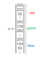
$$({x^{(1)}},{y^{(1)}}),({x^{(2)}},{y^{(2)}}),......,({x^{(m)}},{y^{(m)}})$$
实现方案
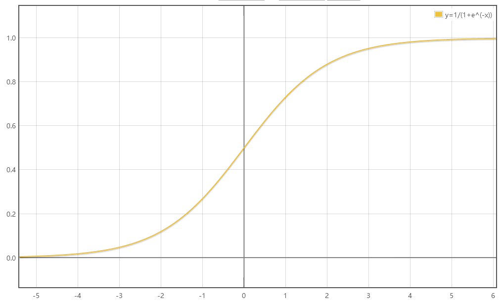
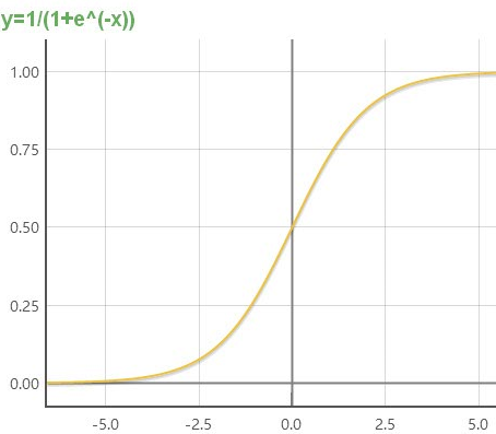
由函数图像可知,sigmoid函数有几个很好的性质:
求参数w和b
使用梯度下降法来求得参数w和b,使得成本函数的最小化
参考学习:http://www.cnblogs.com/pinard/p/5970503.html
在微积分里面,对多元函数的参数求∂偏导数,把求得的各个参数的偏导数以向量的形式写出来,就是梯度。比如函数f(x,y), 分别对x,y求偏导数,求得的梯度向量就是${(\frac{{\partial f}}{{\partial x}},\frac{{\partial f}}{{\partial y}})^T}$,简称grad f(x,y)或者$\nabla f(x,y)$。对于在点(x0,y0)的具体梯度向量就是${(\frac{{\partial f}}{{\partial x_0}},\frac{{\partial f}}{{\partial y_0}})^T}$,或者$\nabla f(x_0,y_0)$,如果是3个参数的向量梯度,就是${(\frac{{\partial f}}{{\partial x}},\frac{{\partial f}}{{\partial y}},\frac{{\partial f}}{{\partial z}})^T}$,以此类推。
那么这个梯度向量求出来有什么意义呢?他的意义从几何意义上讲,就是函数变化增加最快的地方。具体来说,对于函数f(x,y),在点(x0,y0),沿着梯度向量的方向就是$\nabla f(x_0,y_0)$的方向是f(x,y)增加最快的地方。或者说,沿着梯度向量的方向,更加容易找到函数的最大值。反过来说,沿着梯度向量相反的方向,也就是 $-\nabla f(x_0,y_0)$的方向,梯度减少最快,也就是更加容易找到函数的最小值。
在机器学习算法中,在最小化损失函数时,可以通过梯度下降法来一步步的迭代求解,得到最小化的损失函数,和模型参数值(此处即是w和b)。
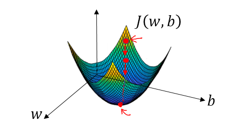
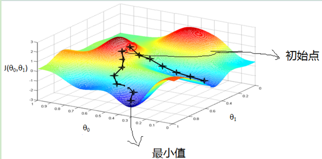
在空间坐标中以w,b为轴画出损失函数J(w,b)的三维图像,可知这个函数为一个凸函数。为了找到合适的参数,先将w和b赋一个初始值,正如图中的小红点。在losgistic回归中,几乎任何初始化方法都有效,通常将参数初始化为零。随机初始化也起作用,但通常不会在losgistic回归中这样做,因为这个成本函数是凸的,无论初始化的值是多少,总会到达同一个点或大致相同的点(最优解)。梯度下降就是从起始点开始,试图在最陡峭的下降方向下坡,以便尽可能快地下坡到达最低点,这个下坡的方向便是此点的梯度值。

在二维图像中来看,顺着导数的方向,下降速度最快,用数学公式表达即是:
$$w: = w - a\frac{{\partial J(w,b)}}{{\partial w}}$$
$$b: = b - a\frac{{\partial J(w,b)}}{{\partial b}}$$
上述两式表示随时更新w与b的值。
待解决问题
Python实现
总代码与输出
#logistic_regression.py
#导入用到的包
import numpy as np
import matplotlib.pyplot as plt
import h5py
import scipy
from PIL import Image
from scipy import ndimage
#导入数据
def load_dataset():
train_dataset = h5py.File("train_cat.h5","r") #读取训练数据,共209张图片
test_dataset = h5py.File("test_cat.h5", "r") #读取测试数据,共50张图片
train_set_x_orig = np.array(train_dataset["train_set_x"][:]) #原始训练集(209*64*64*3)
train_set_y_orig = np.array(train_dataset["train_set_y"][:]) #原始训练集的标签集(y=0非猫,y=1是猫)(209*1)
test_set_x_orig = np.array(test_dataset["test_set_x"][:]) #原始测试集(50*64*64*3
test_set_y_orig = np.array(test_dataset["test_set_y"][:]) #原始测试集的标签集(y=0非猫,y=1是猫)(50*1)
train_set_y_orig = train_set_y_orig.reshape((1,train_set_y_orig.shape[0])) #原始训练集的标签集设为(1*209)
test_set_y_orig = test_set_y_orig.reshape((1,test_set_y_orig.shape[0])) #原始测试集的标签集设为(1*50)
classes = np.array(test_dataset["list_classes"][:])
return train_set_x_orig, train_set_y_orig, test_set_x_orig, test_set_y_orig, classes #classes = [b'non-cat' b'cat']
#显示图片
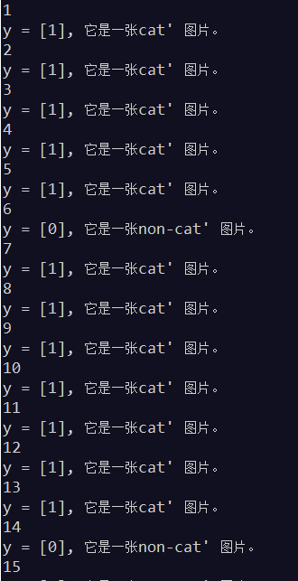
def image_show(index,dataset):
index = index
if dataset == "train":
plt.imshow(train_set_x_orig[index])
print ("y = " + str(train_set_y[:, index]) + ", 它是一张" + classes[np.squeeze(train_set_y[:, index])].decode("utf-8") + "' 图片。")
elif dataset == "load_dataset_test":
plt.imshow(test_set_x_orig[index])
print ("y = " + str(test_set_y[:, index]) + ", 它是一张" + classes[np.squeeze(test_set_y[:, index])].decode("utf-8") + "' 图片。")
#sigmoid函数
def sigmoid(z):
s = 1.0/(1+np.exp(-z))
return s
#初始化参数w,b
def initialize_with_zeros(dim):
w = np.zeros((dim,1)) #w为一个dim*1矩阵
b = 0
return w, b
#计算Y_hat,成本函数J以及dw,db
def propagate(w, b, X, Y):
m = X.shape[1] #样本个数
Y_hat = sigmoid(np.dot(w.T,X)+b)
cost = -(np.sum(np.dot(Y,np.log(Y_hat).T)+np.dot((1-Y),np.log(1-Y_hat).T)))/m #成本函数
dw = (np.dot(X,(Y_hat-Y).T))/m
db = (np.sum(Y_hat-Y))/m
cost = np.squeeze(cost) #压缩维度
grads = {"dw": dw,
"db": db} #梯度
return grads, cost
#梯度下降找出最优解
def optimize(w, b, X, Y, num_iterations, learning_rate, print_cost = False):#num_iterations-梯度下降次数 learning_rate-学习率,即参数ɑ
costs = [] #记录成本值
for i in range(num_iterations): #循环进行梯度下降
grads, cost = propagate(w,b,X,Y)
dw = grads["dw"]
db = grads["db"]
w = w - learning_rate*dw
b = b - learning_rate*db
if i % 100 == 0: #每100次记录一次成本值
costs.append(cost)
if print_cost and i % 100 == 0: #打印成本值
print ("循环%i次后的成本值: %f" %(i, cost))
params = {"w": w,
"b": b} #最终参数值
grads = {"dw": dw,
"db": db}#最终梯度值
return params, grads, costs
#预测出结果
def predict(w, b, X):
m = X.shape[1] #样本个数
Y_prediction = np.zeros((1,m)) #初始化预测输出
w = w.reshape(X.shape[0], 1) #转置参数向量w
Y_hat = sigmoid(np.dot(w.T,X)+b) #最终得到的参数代入方程
for i in range(Y_hat.shape[1]):
if Y_hat[:,i]>0.5:
Y_prediction[:,i] = 1
else:
Y_prediction[:,i] = 0
return Y_prediction
#建立整个预测模型
def model(X_train, Y_train, X_test, Y_test, num_iterations = 2000, learning_rate = 0.5, print_cost = False):
#num_iterations-梯度下降次数 learning_rate-学习率,即参数ɑ
w, b = initialize_with_zeros(X_train.shape[0]) #初始化参数w,b
parameters, grads, costs = optimize(w, b, X_train, Y_train, num_iterations, learning_rate, print_cost) #梯度下降找到最优参数
w = parameters["w"] #获得最终参数
b = parameters["b"] #获得最终参数
Y_prediction_train = predict(w, b, X_train) #训练集的预测结果
Y_prediction_test = predict(w, b, X_test) #测试集的预测结果
train_accuracy = 100 - np.mean(np.abs(Y_prediction_train - Y_train)) * 100 #训练集识别准确度……abs——绝对值……mean——求均值
test_accuracy = 100 - np.mean(np.abs(Y_prediction_test - Y_test)) * 100 #测试集识别准确度
print("训练集识别准确度: {} %".format(train_accuracy))
print("测试集识别准确度: {} %".format(test_accuracy))
d = {"costs": costs,
"Y_prediction_test": Y_prediction_test,
"Y_prediction_train" : Y_prediction_train,
"w" : w,
"b" : b,
"learning_rate" : learning_rate,
"num_iterations": num_iterations}
return d
#初始化数据
train_set_x_orig, train_set_y, test_set_x_orig, test_set_y, classes = load_dataset()
m_train = train_set_x_orig.shape[0] #训练集中样本个数
m_test = test_set_x_orig.shape[0] #测试集总样本个数
num_px = test_set_x_orig.shape[1] #图片的像素大小
train_set_x_flatten = train_set_x_orig.reshape(train_set_x_orig.shape[0],-1).T #原始训练集的设为(12288*209)
test_set_x_flatten = test_set_x_orig.reshape(test_set_x_orig.shape[0],-1).T #原始测试集设为(12288*50)
train_set_x = train_set_x_flatten/255. #将训练集矩阵标准化
test_set_x = test_set_x_flatten/255. #将测试集矩阵标准化
d = model(train_set_x, train_set_y, test_set_x, test_set_y, num_iterations = 2000, learning_rate = 0.005, print_cost = True)
# 画出学习曲线
costs = np.squeeze(d['costs'])
plt.plot(costs)
plt.ylabel('cost')
plt.xlabel('iterations (per hundreds)')
plt.title("Learning rate =" + str(d["learning_rate"]))
plt.show()
#学习率不同时的学习曲线
learning_rates = [0.01, 0.001, 0.0001]
models = {}
for i in learning_rates:
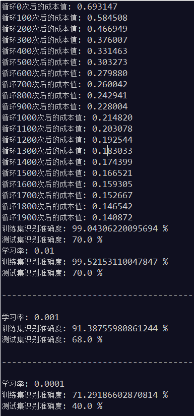
print ("学习率: " + str(i))
models[str(i)] = model(train_set_x, train_set_y, test_set_x, test_set_y, num_iterations = 2000, learning_rate = i, print_cost = False)
print ('\n' + "-------------------------------------------------------" + '\n')
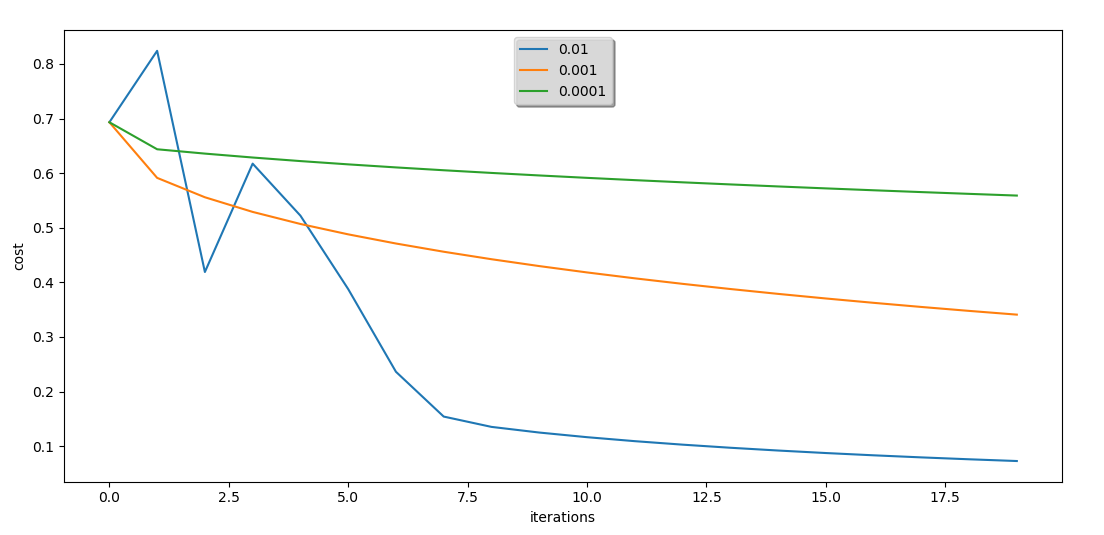
for i in learning_rates:
plt.plot(np.squeeze(models[str(i)]["costs"]), label= str(models[str(i)]["learning_rate"]))
plt.ylabel('cost')
plt.xlabel('iterations')
legend = plt.legend(loc='upper center', shadow=True)
frame = legend.get_frame()
frame.set_facecolor('0.90')
plt.show()
out:
解释:
以上输出表示的是梯度下降次数为2000次,每次的下降步长分别为0.01,,0.001,0.0001的测试结果。
由测试结果可知:
1、循环n次后的成本值最小可以达到为0,而成本值表示的是预测值与真实值之间的差异程度,差异越小越好,所以达到为0 是最理想的结果。
2、梯度下降的次数与下降步长需要协调改进,如同你要走一段固定的距离到达一个位置(即达到成本值最小,但具体不知道多少),步数多了,步子就要变小,步数少了,步子就要变大,但其实我们总有可能还没有到达那个位置或者超过了那个位置。以上测试中只减小了步长,很大可能是成本值还没有达到最小值。
3、训练集的准确度是可以达到100%的,因为我们是通过训练集来确定出算法参数的,也即是说训练集的数据必然是接近100%拟合算法的,但测试集不是,测试集是我们确定了算法之后,再将经过算法得出的的预测值与真实值进行比较得到的结果。
函数汇总
- load_dataset():return train_set_x_orig, train_set_y_orig, test_set_x_orig, test_set_y_orig, classes #导入数据
- image_show(index,dataset):return null #显示图片
- sigmoid(z):return s #sigmoid函数
- initialize_with_zeros(dim):return w, b ##初始化参数w,b
- propagate(w, b, X, Y):return grads, cost ##计算Y_hat,成本函数J以及dw,db
- optimize(w, b, X, Y, num_iterations, learning_rate, print_cost = False):return params, grads, costs #梯度下降找出最优解
- predict(w, b, X):return Y_prediction #预测出结果
- model(X_train, Y_train, X_test, Y_test, num_iterations = 2000, learning_rate = 0.5, print_cost = False):return d #建立整个预测模型
整个算法大概的流程:导入数据load_dataset()——通过训练数据计算$\hat y$propagate(w, b, X, Y),该函数会返回w和b的梯度值与成本函数cost公式——通过梯度下降法找出w和b的最优解optimize( ),返回最终的w和b参数——再把w和b参数赋给函数predict(),得出最终的预测算法
以上流程部分嵌套,最后整合在model()中.
部分代码分块解释
数据导入load_dataset():(加入了测试代码)
#logistic_regression.py
#导入用到的包
import numpy as np
import matplotlib.pyplot as plt
import h5py
import scipy
from PIL import Image
from scipy import ndimage
#导入数据
def load_dataset():
train_dataset = h5py.File("train_cat.h5","r") #读取训练数据,共209张图片
test_dataset = h5py.File("test_cat.h5", "r") #读取测试数据,共50张图片
train_set_x_orig = np.array(train_dataset["train_set_x"][:]) #原始训练集(209*64*64*3)
train_set_y_orig = np.array(train_dataset["train_set_y"][:]) #原始训练集的标签集(y=0非猫,y=1是猫)(209*1)
test_set_x_orig = np.array(test_dataset["test_set_x"][:]) #原始测试集(50*64*64*3
test_set_y_orig = np.array(test_dataset["test_set_y"][:]) #原始测试集的标签集(y=0非猫,y=1是猫)(50*1)
train_set_y_orig = train_set_y_orig.reshape((1,train_set_y_orig.shape[0])) #原始训练集的标签集设为(1*209)
test_set_y_orig = test_set_y_orig.reshape((1,test_set_y_orig.shape[0])) #原始测试集的标签集设为(1*50)
classes = np.array(test_dataset["list_classes"][:])
return train_set_x_orig, train_set_y_orig, test_set_x_orig, test_set_y_orig, classes
#初始化数据
train_set_x_orig, train_set_y, test_set_x_orig, test_set_y, classes = load_dataset() #classes = [b'non-cat' b'cat']
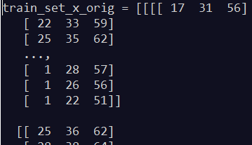
#print("train_set_x_orig = " + str(train_set_x_orig))
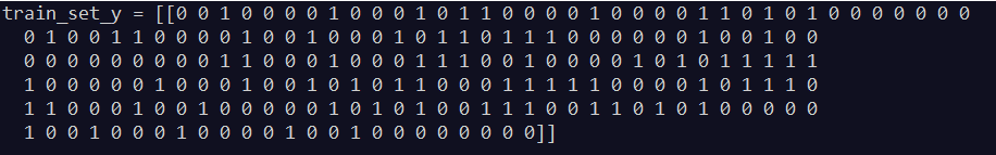
#print("train_set_y = " + str(train_set_y))
#print("test_set_x_orig = " + str(test_set_x_orig))
#print("test_set_y = " + str(test_set_y))
print("classes = " + str(classes))
#print("type(train_set_x_orig) = " + str(type(train_set_x_orig)))
#print("type(train_set_y) = " + str(type(train_set_y)))
测试:
print("type(train_set_y) = " + str(type(train_set_y)))————输出:type(train_set_y) = <class 'numpy.ndarray'>:输出的数据是数组形式
如下(图片数据的保存形式,即.h5文件内容):
print("classes = " + str(classes))————输出: classes = [b'non-cat' b'cat']
将数据还原为图片:
#logistic_regression.py
#导入用到的包
import numpy as np
import matplotlib.pyplot as plt
import h5py
import scipy
from PIL import Image
from scipy import ndimage
#导入数据
def load_dataset():
train_dataset = h5py.File("train_cat.h5","r") #读取训练数据,共209张图片
test_dataset = h5py.File("test_cat.h5", "r") #读取测试数据,共50张图片
train_set_x_orig = np.array(train_dataset["train_set_x"][:]) #原始训练集(209*64*64*3)
train_set_y_orig = np.array(train_dataset["train_set_y"][:]) #原始训练集的标签集(y=0非猫,y=1是猫)(209*1)
test_set_x_orig = np.array(test_dataset["test_set_x"][:]) #原始测试集(50*64*64*3
test_set_y_orig = np.array(test_dataset["test_set_y"][:]) #原始测试集的标签集(y=0非猫,y=1是猫)(50*1)
train_set_y_orig = train_set_y_orig.reshape((1,train_set_y_orig.shape[0])) #原始训练集的标签集设为(1*209)
test_set_y_orig = test_set_y_orig.reshape((1,test_set_y_orig.shape[0])) #原始测试集的标签集设为(1*50)
classes = np.array(test_dataset["list_classes"][:])
return train_set_x_orig, train_set_y_orig, test_set_x_orig, test_set_y_orig, classes
#显示图片
def image_show(index,dataset):
index = index
if dataset == "train":
plt.imshow(train_set_x_orig[index])
print ("y = " + str(train_set_y[:, index]) + ", 它是一张" + classes[np.squeeze(train_set_y[:, index])].decode("utf-8") + "' 图片。")
elif dataset == "load_dataset_test":
plt.imshow(test_set_x_orig[index])
print ("y = " + str(test_set_y[:, index]) + ", 它是一张" + classes[np.squeeze(test_set_y[:, index])].decode("utf-8") + "' 图片。")
#初始化数据
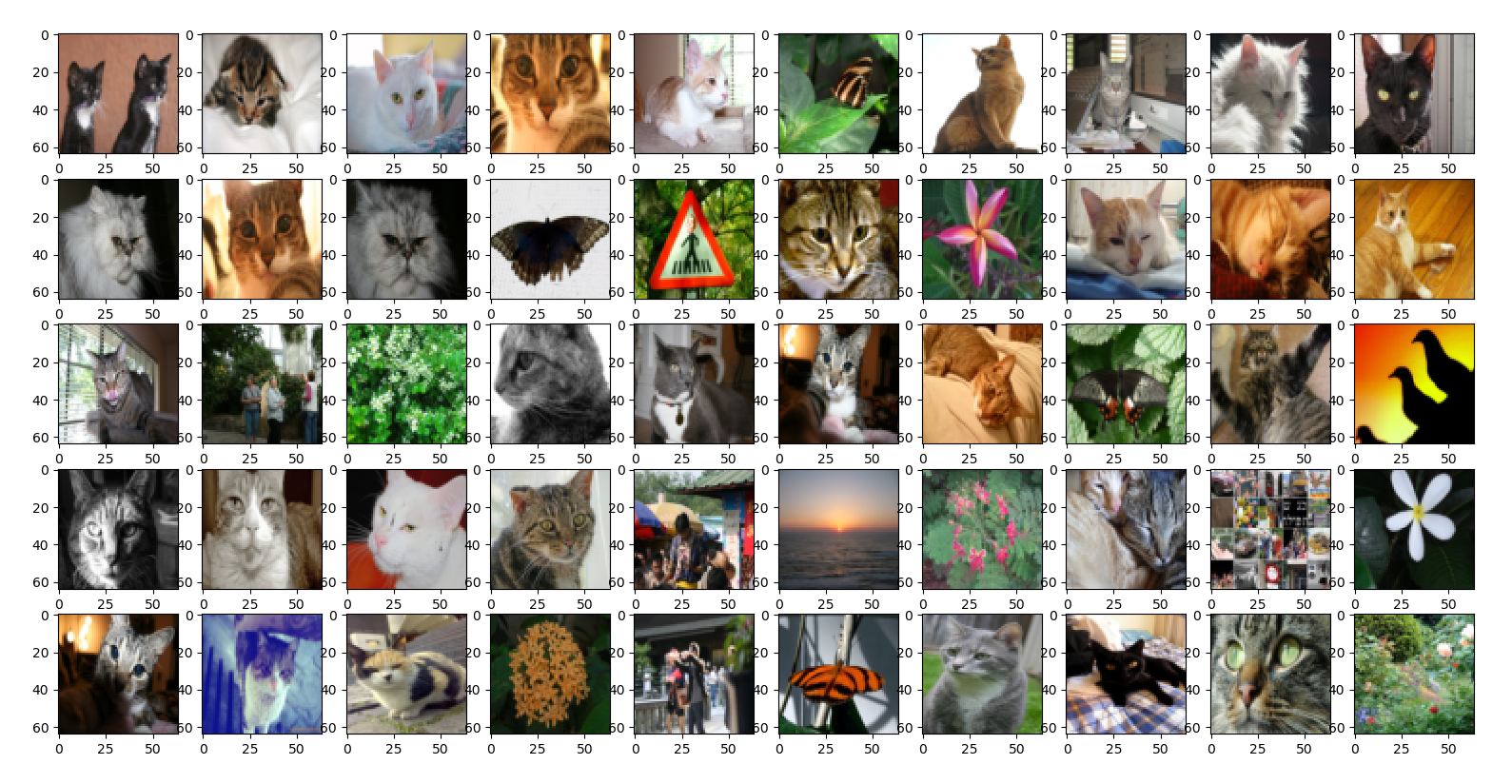
train_set_x_orig, train_set_y, test_set_x_orig, test_set_y, classes = load_dataset()
for i in range(0,50):
plt.subplot(5,10,i+1)
print(i+1)
image_show(i,"load_dataset_test")
plt.show()
'''
for i in range(0,50):
plt.subplot(5,10,i+1)
print(i+1)
image_show(i,"train")
plt.show()
'''

输出:
关于最优解
来看看梯度下降的一个直观的解释。比如我们在一座大山上的某处位置,由于我们不知道怎么下山,于是决定走一步算一步,也就是在每走到一个位置的时候,求解当前位置的梯度,沿着梯度的负方向,也就是当前最陡峭的位置向下走一步,然后继续求解当前位置梯度,向这一步所在位置沿着最陡峭最易下山的位置走一步。这样一步步的走下去,一直走到觉得我们已经到了山脚。当然这样走下去,有可能我们不能走到山脚,而是到了某一个局部的山峰低处。
从上面的解释可以看出,梯度下降不一定能够找到全局的最优解,有可能是一个局部最优解。当然,如果损失函数是凸函数,梯度下降法得到的解就一定是全局最优解。
来源:http://www.cnblogs.com/pinard/p/5970503.html
关于sigmoid函数中e的参数对算法结果的影响
不同a值情况下的图像
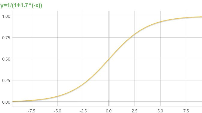

在程序中改变a的值进行测试
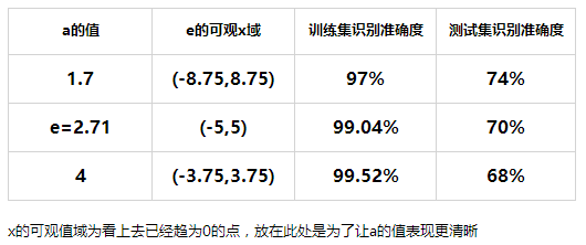
以上的结果是在梯度下降次数为2000次,学习率为0.005的条件下测试的,可以看出,调整a的值是有助于改变识别准确度的。
但也可以看到,在相同条件下,只改变a的值也会改变训练集的识别准确度,这又是为什么?
我们知道训练集的识别准确度是可以通过梯度下降次数与学习率的调整最高达到100%的,那么再测试一下不同梯度下降次数条件下识别的准确度会有什么影响:

由以上测试可以看出,训练集的识别准确度是可以达到100%的,但相应的却降低了测试集的识别准确度。
我们知道训练集的准确度可以达到100%,完全是因为算法的参数就是从中计算出来的,也就是说,训练集的数据是近乎完全拟合算法的。但测试集不是,我们只是找了另外一些数据来对得到的这个算法进行测试,测试的过程类似于我们拿两张猫的图片来进行对比,一张已知是猫,一张未知,看他们的相似程度,相似程度高,就认为未知图片是猫。只是算法换成了数据,对比的也是数据。先把数据转换成函数,再通过这个函数来测试另外的数据。但就是这个数据转换成函数的结果,有很多种,优劣不一,它必然会省略掉一些信息,导致另外拿来测试的数据实际上应该是符合的却被测试为不符合。也即是再好的一个识别猫的算法,我们必然有可能拿一张不是猫的图像让它认为是猫,再拿一张是猫的图像让它认为不是猫(也即是对抗样本模型)。
所以说,上面测试集识别准确度与训练集准确度的关系并不会是线性的,跟算法有很大的关系,但即使如此,测试集的识别准确度也在68%-74%之间了(梯度优化足够的前提下)。