TensorFlow中设置学习率的方式
学习率α需要在训练之前指定,学习率设定的重要性不言而喻:过小的学习率会降低网络优化的速度,增加训练时间;而过大的学习率则可能导致最后的结果不会收敛,或者在一个较大的范围内摆动;因此,在训练的过程中,根据训练的迭代次数调整学习率的大小,是非常有必要的
本主要主要介绍的学习率设置方式有:
- 指数衰减: tf.train.exponential_decay()
- 分段常数衰减: tf.train.piecewise_constant()
- 自然指数衰减: tf.train.natural_exp_decay()
- 多项式衰减tf.train.polynomial_decay()
- 倒数衰减tf.train.inverse_time_decay()
- 余弦衰减tf.train.cosine_decay()
指数衰减
1 tf.train.exponential_decay(
2     learning_rate,
3     global_step,
4     decay_steps,
5     decay_rate,
6     staircase=False,
7     name=None):
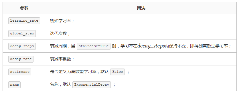
计算方式:
1 decayed_learning_rate = learning_rate * decay_rate ^ (global_step / decay_steps)
2 # 如果staircase=True,则学习率会在得到离散值,每decay_steps迭代次数,更新一次;
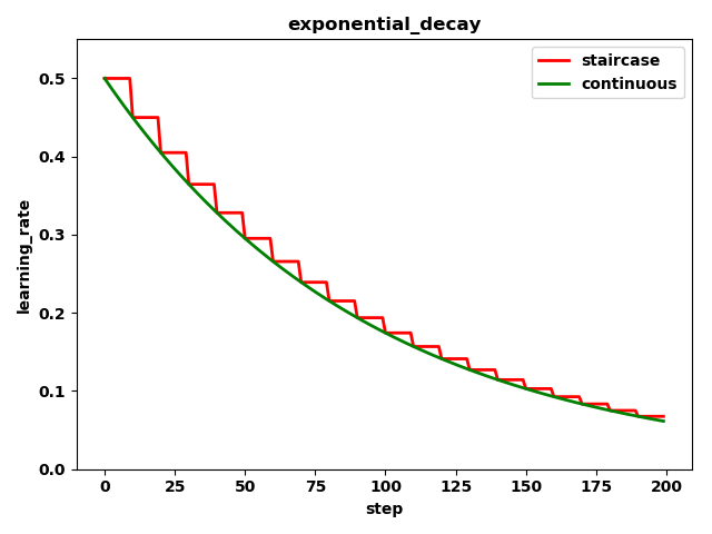
示例:
 1 import matplotlib.pyplot as plt
 2 import tensorflow as tf
 3
 4 global_step = tf.Variable(0, name='global_step', trainable=False) # 迭代次数
 5
 6 y = []
 7 z = []
 8 epochs = 200
 9
10 with tf.Session() as sess:
11     sess.run(tf.global_variables_initializer())
12     for global_step in range(epochs):
13         # 阶梯型衰减
14         learning_rate_1 = tf.train.exponential_decay(
15             learning_rate=0.5, global_step=global_step, decay_steps=10, decay_rate=0.9, staircase=True
16         )
17         # 标准指数衰减
18         learning_rate_2 = tf.train.exponential_decay(
19             learning_rate=0.5, global_step=global_step, decay_steps=10, decay_rate=0.9, staircase=False
20         )
21         lr1 = sess.run([learning_rate_1])
22         lr2 = sess.run([learning_rate_2])
23         y.append(lr1)
24         z.append(lr2)
25
26 x = range(epochs)
27 fig = plt.figure()
28 ax = fig.add_subplot(111)
29 ax.set_ylim([0, 0.55])
30
31 plt.plot(x, y, 'r-', linewidth=2)
32 plt.plot(x, z, 'g-', linewidth=2)
33 plt.title('exponential_decay')
34 ax.set_xlabel('step')
35 ax.set_ylabel('learning_rate')
36 plt.legend(labels=['staircase', 'continuous'], loc='upper right')
37 plt.show()
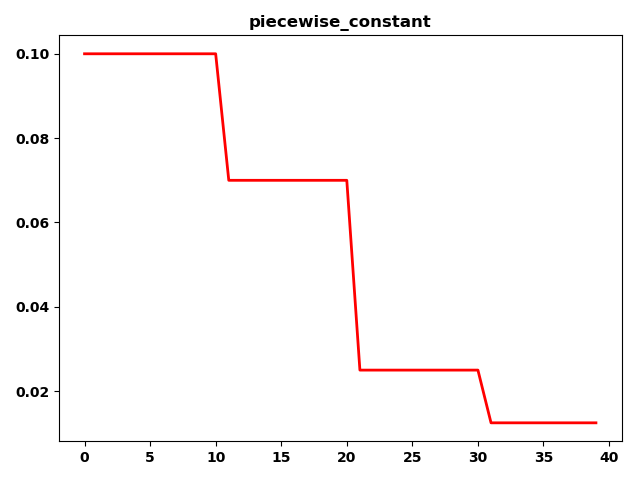
分段常数衰减
1 tf.train.piecewise_constant(
2     x,
3     boundaries,
4     values,
5     name=None):

计算方式:
 1 # parameter
 2 global_step = tf.Variable(0, trainable=False)
 3 boundaries = [100, 200]
 4 values = [1.0, 0.5, 0.1]
 5 # learning_rate
 6 learning_rate = tf.train.piecewise_constant(global_step, boundaries, values)
 7 # 解释
 8 # 当global_step=[1, 100]时,learning_rate=1.0;
 9 # 当global_step=[101, 200]时,learning_rate=0.5;
10 # 当global_step=[201, ~]时,learning_rate=0.1;
示例:
 1 import matplotlib.pyplot as plt
 2 import tensorflow as tf
 3
 4 global_step = tf.Variable(0, name='global_step', trainable=False) # 迭代次数
 5 boundaries = [10, 20, 30]
 6 learning_rates = [0.1, 0.07, 0.025, 0.0125]
 7
 8 y = []
 9 N = 40
10
11 with tf.Session() as sess:
12     sess.run(tf.global_variables_initializer())
13     for global_step in range(N):
14         learning_rate = tf.train.piecewise_constant(global_step, boundaries=boundaries, values=learning_rates)
15         lr = sess.run([learning_rate])
16         y.append(lr)
17
18 x = range(N)
19 plt.plot(x, y, 'r-', linewidth=2)
20 plt.title('piecewise_constant')
21 plt.show()
自然指数衰减
类似与指数衰减,同样与当前迭代次数相关,只不过以e为底;
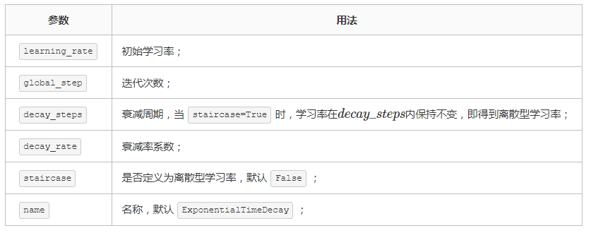
1 tf.train.natural_exp_decay(
2     learning_rate,
3     global_step,
4     decay_steps,
5     decay_rate,
6     staircase=False,
7     name=None
8 )
计算方式:
1 decayed_learning_rate = learning_rate * exp(-decay_rate * global_step)
2 # 如果staircase=True,则学习率会在得到离散值,每decay_steps迭代次数,更新一次;
示例:
 1 import matplotlib.pyplot as plt
 2 import tensorflow as tf
 3
 4 global_step = tf.Variable(0, name='global_step', trainable=False)
 5
 6 y = []
 7 z = []
 8 w = []
 9 m = []
10 EPOCH = 200
11
12 with tf.Session() as sess:
13     sess.run(tf.global_variables_initializer())
14     for global_step in range(EPOCH):
15
16         # 阶梯型衰减
17         learning_rate1 = tf.train.natural_exp_decay(
18             learning_rate=0.5, global_step=global_step, decay_steps=10, decay_rate=0.9, staircase=True)
19
20         # 标准指数型衰减
21         learning_rate2 = tf.train.natural_exp_decay(
22             learning_rate=0.5, global_step=global_step, decay_steps=10, decay_rate=0.9, staircase=False)
23
24         # 阶梯型指数衰减
25         learning_rate3 = tf.train.exponential_decay(
26             learning_rate=0.5, global_step=global_step, decay_steps=10, decay_rate=0.9, staircase=True)
27
28         # 标准指数衰减
29         learning_rate4 = tf.train.exponential_decay(
30             learning_rate=0.5, global_step=global_step, decay_steps=10, decay_rate=0.9, staircase=False)
31
32         lr1 = sess.run([learning_rate1])
33         lr2 = sess.run([learning_rate2])
34         lr3 = sess.run([learning_rate3])
35         lr4 = sess.run([learning_rate4])
36
37         y.append(lr1)
38         z.append(lr2)
39         w.append(lr3)
40         m.append(lr4)
41
42 x = range(EPOCH)
43 fig = plt.figure()
44 ax = fig.add_subplot(111)
45 ax.set_ylim([0, 0.55])
46
47 plt.plot(x, y, 'r-', linewidth=2)
48 plt.plot(x, z, 'g-', linewidth=2)
49 plt.plot(x, w, 'r--', linewidth=2)
50 plt.plot(x, m, 'g--', linewidth=2)
51
52 plt.title('natural_exp_decay')
53 ax.set_xlabel('step')
54 ax.set_ylabel('learning rate')
55 plt.legend(labels = ['natural_staircase', 'natural_continuous', 'staircase', 'continuous'], loc = 'upper right')
56 plt.show()
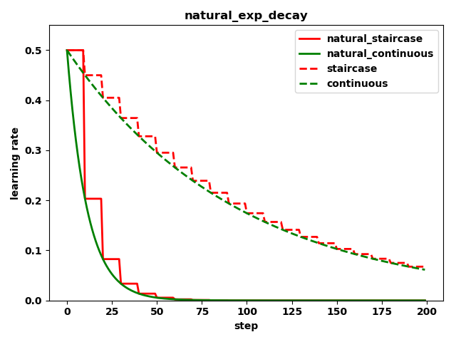
可以看到自然指数衰减对学习率的衰减程度远大于一般的指数衰减;
多项式衰减
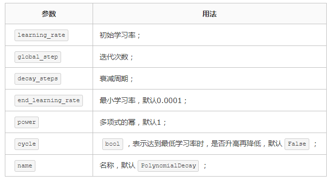
1 tf.train.polynomial_decay(
2     learning_rate,
3     global_step,
4     decay_steps,
5     end_learning_rate=0.0001,
6     power=1.0,
7     cycle=False, name=None):
计算方式:
 1 # 如果cycle=False
 2 global_step = min(global_step, decay_steps)
 3 decayed_learning_rate = (learning_rate - end_learning_rate) *
 4                           (1 - global_step / decay_steps) ^ (power) +
 5                           end_learning_rate
 6 # 如果cycle=True
 7 decay_steps = decay_steps * ceil(global_step / decay_steps)
 8 decayed_learning_rate = (learning_rate - end_learning_rate) *
 9                           (1 - global_step / decay_steps) ^ (power) +
10                           end_learning_rate
示例:
 1 import matplotlib.pyplot as plt
 2 import tensorflow as tf
 3
 4 y = []
 5 z = []
 6 EPOCH = 200
 7
 8 global_step = tf.Variable(0, name='global_step', trainable=False)
 9
10 with tf.Session() as sess:
11     sess.run(tf.global_variables_initializer())
12     for global_step in range(EPOCH):
13         # cycle=False
14         learning_rate1 = tf.train.polynomial_decay(
15             learning_rate=0.1, global_step=global_step, decay_steps=50,
16             end_learning_rate=0.01, power=0.5, cycle=False)
17         # cycle=True
18         learning_rate2 = tf.train.polynomial_decay(
19             learning_rate=0.1, global_step=global_step, decay_steps=50,
20             end_learning_rate=0.01, power=0.5, cycle=True)
21
22         lr1 = sess.run([learning_rate1])
23         lr2 = sess.run([learning_rate2])
24         y.append(lr1)
25         z.append(lr2)
26
27 x = range(EPOCH)
28 fig = plt.figure()
29 ax = fig.add_subplot(111)
30 plt.plot(x, z, 'g-', linewidth=2)
31 plt.plot(x, y, 'r--', linewidth=2)
32 plt.title('polynomial_decay')
33 ax.set_xlabel('step')
34 ax.set_ylabel('learning rate')
35 plt.legend(labels=['cycle=True', 'cycle=False'], loc='upper right')
36 plt.show()
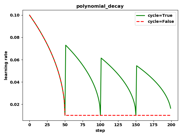
可以看到学习率在decay_steps=50迭代次数后到达最小值;同时,当cycle=False时,学习率达到预设的最小值后,就保持最小值不再变化;当cycle=True时,学习率将会瞬间增大,再降低;
多项式衰减中设置学习率可以往复升降的目的:时为了防止在神经网络训练后期由于学习率过小,导致网络参数陷入局部最优,将学习率升高,有可能使其跳出局部最优;
倒数衰减
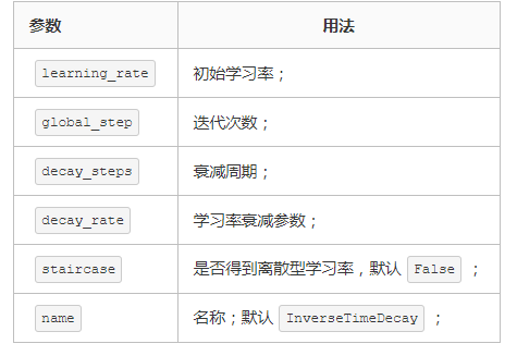
1 inverse_time_decay(
2     learning_rate,
3     global_step,
4     decay_steps,
5     decay_rate,
6     staircase=False,
7     name=None):
计算方式:
1 # 如果staircase=False,即得到连续型衰减学习率;
2 decayed_learning_rate = learning_rate / (1 + decay_rate * global_step / decay_step)
3
4 # 如果staircase=True,即得到离散型衰减学习率;
5 decayed_learning_rate = learning_rate / (1 + decay_rate * floor(global_step / decay_step))
示例:
 1 import matplotlib.pyplot as plt
 2 import tensorflow as tf
 3
 4 y = []
 5 z = []
 6 EPOCH = 200
 7 global_step = tf.Variable(0, name='global_step', trainable=False)
 8
 9 with tf.Session() as sess:
10     sess.run(tf.global_variables_initializer())
11     for global_step in range(EPOCH):
12         # 阶梯型衰减
13         learning_rate1 = tf.train.inverse_time_decay(
14             learning_rate=0.1, global_step=global_step, decay_steps=20,
15             decay_rate=0.2, staircase=True)
16
17         # 连续型衰减
18         learning_rate2 = tf.train.inverse_time_decay(
19             learning_rate=0.1, global_step=global_step, decay_steps=20,
20             decay_rate=0.2, staircase=False)
21
22         lr1 = sess.run([learning_rate1])
23         lr2 = sess.run([learning_rate2])
24
25         y.append(lr1)
26         z.append(lr2)
27
28 x = range(EPOCH)
29 fig = plt.figure()
30 ax = fig.add_subplot(111)
31 plt.plot(x, z, 'r-', linewidth=2)
32 plt.plot(x, y, 'g-', linewidth=2)
33 plt.title('inverse_time_decay')
34 ax.set_xlabel('step')
35 ax.set_ylabel('learning rate')
36 plt.legend(labels=['continuous', 'staircase'])
37 plt.show()
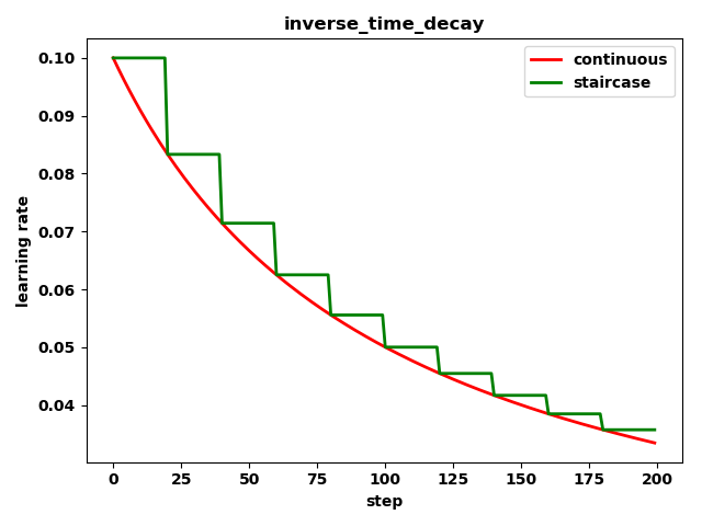
同样可以看到,随着迭代次数的增加,学习率在逐渐减小,同时减小的幅度也在降低;
余弦衰减
1. 标准余弦衰减
1 tf.train.cosine_decay(
2     learning_rate,
3     global_step,
4     decay_steps,
5     alpha=0.0,
6     name=None):

计算方式:
1 global_step = min(global_step, decay_steps)
2 cosine_decay = 0.5 * (1 + cos(pi * global_step / decay_steps))
3 decayed = (1 - alpha) * cosine_decay + alpha
4 decayed_learning_rate = learning_rate * decayed
示例:
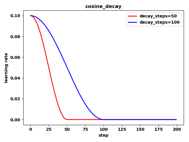
 1 import matplotlib.pyplot as plt
 2 import tensorflow as tf
 3
 4 y = []
 5 z = []
 6 EPOCH = 200
 7 global_step = tf.Variable(0, name='global_step', trainable=False)
 8
 9 with tf.Session() as sess:
10     sess.run(tf.global_variables_initializer())
11     for global_step in range(EPOCH):
12         # 余弦衰减
13         learning_rate1 = tf.train.cosine_decay(
14             learning_rate=0.1, global_step=global_step, decay_steps=50)
15         learning_rate2 = tf.train.cosine_decay(
16             learning_rate=0.1, global_step=global_step, decay_steps=100)
17
18         lr1 = sess.run([learning_rate1])
19         lr2 = sess.run([learning_rate2])
20         y.append(lr1)
21         z.append(lr2)
22
23 x = range(EPOCH)
24 fig = plt.figure()
25 ax = fig.add_subplot(111)
26 plt.plot(x, y, 'r-', linewidth=2)
27 plt.plot(x, z, 'b-', linewidth=2)
28 plt.title('cosine_decay')
29 ax.set_xlabel('step')
30 ax.set_ylabel('learning rate')
31 plt.legend(labels=['decay_steps=50', 'decay_steps=100'], loc='upper right')
32 plt.show()
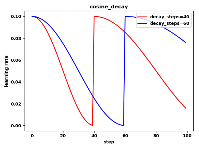
2.重启余弦衰减
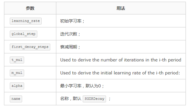
1 tf.train.cosine_decay_restarts(
2     learning_rate,
3     global_step,
4     first_decay_steps,
5     t_mul=2.0,
6     m_mul=1.0,
7     alpha=0.0,
8     name=None):
示例:
 1 import matplotlib.pyplot as plt
 2 import tensorflow as tf
 3
 4 y = []
 5 z = []
 6 EPOCH = 100
 7 global_step = tf.Variable(0, name='global_step', trainable=False)
 8
 9 with tf.Session() as sess:
10     sess.run(tf.global_variables_initializer())
11     for global_step in range(EPOCH):
12         # 重启余弦衰减
13         learning_rate1 = tf.train.cosine_decay_restarts(learning_rate=0.1, global_step=global_step,
14                                            first_decay_steps=40)
15         learning_rate2 = tf.train.cosine_decay_restarts(learning_rate=0.1, global_step=global_step,
16                                                        first_decay_steps=60)
17
18         lr1 = sess.run([learning_rate1])
19         lr2 = sess.run([learning_rate2])
20         y.append(lr1)
21         z.append(lr2)
22
23 x = range(EPOCH)
24 fig = plt.figure()
25 ax = fig.add_subplot(111)
26 plt.plot(x, y, 'r-', linewidth=2)
27 plt.plot(x, z, 'b-', linewidth=2)
28 plt.title('cosine_decay')
29 ax.set_xlabel('step')
30 ax.set_ylabel('learning rate')
31 plt.legend(labels=['decay_steps=40', 'decay_steps=60'], loc='upper right')
32 plt.show()
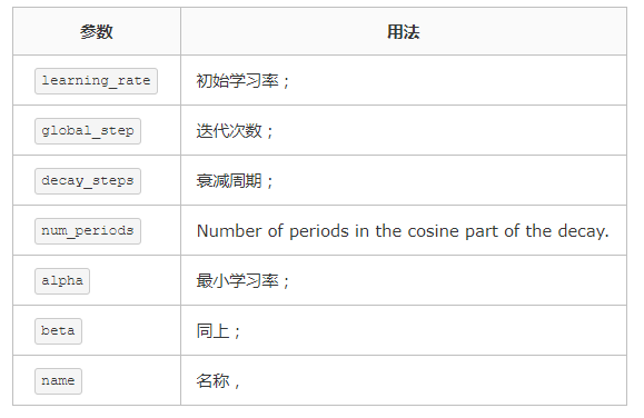
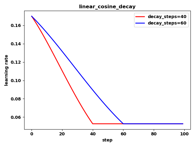
3. 线性余弦噪声
1 tf.train.linear_cosine_decay(
2     learning_rate,
3     global_step,
4     decay_steps,
5     num_periods=0.5,
6     alpha=0.0,
7     beta=0.001,
8     name=None):
计算方式:
1 global_step = min(global_step, decay_steps)
2 linear_decay = (decay_steps - global_step) / decay_steps)
3 cosine_decay = 0.5 * (1 + cos(pi * 2 * num_periods * global_step / decay_steps))
4 decayed = (alpha + linear_decay) * cosine_decay + beta
5 decayed_learning_rate = learning_rate * decayed
示例:
 1 import matplotlib.pyplot as plt
 2 import tensorflow as tf
 3
 4 y = []
 5 z = []
 6 EPOCH = 100
 7 global_step = tf.Variable(0, name='global_step', trainable=False)
 8
 9 with tf.Session() as sess:
10     sess.run(tf.global_variables_initializer())
11     for global_step in range(EPOCH):
12         # 线性余弦衰减
13         learing_rate1 = tf.train.linear_cosine_decay(
14             learning_rate=0.1, global_step=global_step, decay_steps=40,
15             num_periods=0.2, alpha=0.5, beta=0.2)
16         learing_rate2 = tf.train.linear_cosine_decay(
17             learning_rate=0.1, global_step=global_step, decay_steps=60,
18             num_periods=0.2, alpha=0.5, beta=0.2)
19
20         lr1 = sess.run([learing_rate1])
21         lr2 = sess.run([learing_rate2])
22         y.append(lr1)
23         z.append(lr2)
24
25
26 x = range(EPOCH)
27 fig = plt.figure()
28 ax = fig.add_subplot(111)
29 plt.plot(x, y, 'r-', linewidth=2)
30 plt.plot(x, z, 'b-', linewidth=2)
31 plt.title('linear_cosine_decay')
32 ax.set_xlabel('step')
33 ax.set_ylabel('learing rate')
34 plt.legend(labels=['decay_steps=40', 'decay_steps=60'], loc='upper right')
35 plt.show()
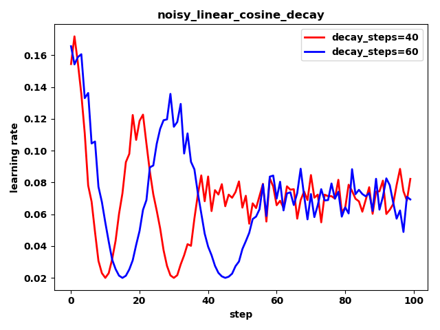
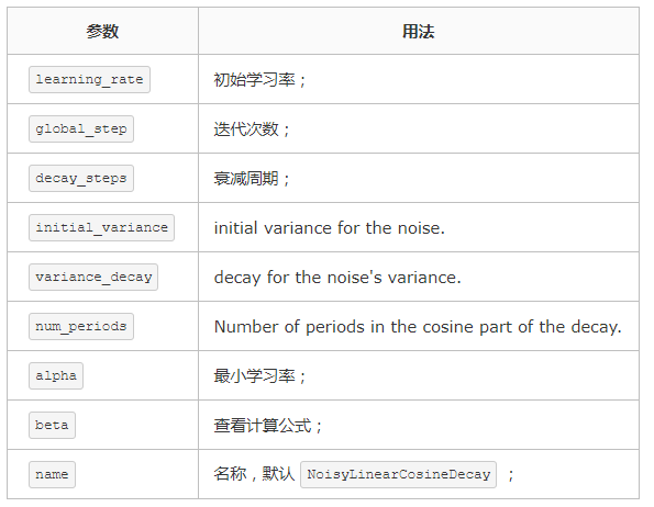
4.噪声余弦衰减
 1 tf.train.noisy_linear_cosine_decay(
 2     learning_rate,
 3     global_step,
 4     decay_steps,
 5     initial_variance=1.0,
 6     variance_decay=0.55,
 7     num_periods=0.5,
 8     alpha=0.0,
 9     beta=0.001,
10     name=None):
计算方式:
1 global_step = min(global_step, decay_steps)
2 linear_decay = (decay_steps - global_step) / decay_steps)
3 cosine_decay = 0.5 * (
4     1 + cos(pi * 2 * num_periods * global_step / decay_steps))
5 decayed = (alpha + linear_decay + eps_t) * cosine_decay + beta
6 decayed_learning_rate = learning_rate * decayed
示例:
 1 import matplotlib.pyplot as plt
 2 import tensorflow as tf
 3
 4 y = []
 5 z = []
 6 EPOCH = 100
 7 global_step = tf.Variable(0, name='global_step', trainable=False)
 8
 9 with tf.Session() as sess:
10     sess.run(tf.global_variables_initializer())
11     for global_step in range(EPOCH):
12         # # 噪声线性余弦衰减
13         learning_rate1 = tf.train.noisy_linear_cosine_decay(
14             learning_rate=0.1, global_step=global_step, decay_steps=40,
15             initial_variance=0.01, variance_decay=0.1, num_periods=2, alpha=0.5, beta=0.2)
16         learning_rate2 = tf.train.noisy_linear_cosine_decay(
17             learning_rate=0.1, global_step=global_step, decay_steps=60,
18             initial_variance=0.01, variance_decay=0.1, num_periods=2, alpha=0.5, beta=0.2)
19
20         lr1 = sess.run([learning_rate1])
21         lr2 = sess.run([learning_rate2])
22         y.append(lr1)
23         z.append(lr2)
24
25 x = range(EPOCH)
26 fig = plt.figure()
27 ax = fig.add_subplot(111)
28 plt.plot(x, y, 'r-', linewidth=2)
29 plt.plot(x, z, 'b-', linewidth=2)
30 plt.title('noisy_linear_cosine_decay')
31 ax.set_xlabel('step')
32 ax.set_ylabel('learning rate')
33 plt.legend(labels=['decay_steps=40', 'decay_steps=60'], loc='upper right')
34 plt.show()