【机器学习】拟合一元二次方程
多项式回归实现
实验目的
基于单变量线性回归模型实现拟合一个多项式函数
\[y = ax^2 + bx + c
\]
需要实现的函数
compute_model_output: 计算 \(y = ax^2 + bx + c\) 的值compute_cost: 计算一组 a,b 的均方误差compute_gradient: 计算偏导数gradient_descent: 梯度下降算法- 绘制图像
数学公式推导
数学模型:
\[f_{a,b,c}(x) = ax^2 + bx +c \tag{1}
\]
损失函数
与单源线性回归相同,采用均方误差来作为损失函数
\[J(a,b,c) = \frac{1}{2m} \sum_{i=0}^{m-1}(f_{a,b,c}(x^{(i)}) - y^{(i)})^2 \tag{2}
\]
\[f_{a,b,c}(x^{(i)} = a(x^{(i)})^{2} + bx^{(i)} + c \tag{3}
\]
梯度计算
\[\begin{align}
\frac{\partial J(a,b,c)}{\partial a} &= \frac{1}{m} \sum_{i=0}^{m-1}(f_{a,b,c}(x^{(i)}) - y^{(i)})(x^{(i)})^2 \tag{4}\\
\frac{\partial J(a,b,c)}{\partial b} &= \frac{1}{m} \sum_{i=0}^{m-1}(f_{a,b,c}(x^{(i)}) - y^{(i)})x^{(i)} \tag{5}\\
\frac{\partial J(a,b,c)}{\partial c} &= \frac{1}{m} \sum_{i=0}^{m-1}(f_{a,b,c}(x^{(i)}) - y^{(i)}) \tag{6} \\
\end{align}
\]
梯度下降算法
\[\begin{align*}
\text{repeat}&\text{ until convergence:} \; \lbrace \\
a &= a - \alpha \frac{\partial J(a,b,c)}{\partial w} \tag{7} \\
b &= b - \alpha \frac{\partial J(a,b,c)}{\partial b} \\
c &= c - \alpha \frac{\partial J(a,b,c)}{\partial c} \\
\rbrace
\end{align*}
\]
遇到的问题
-
在
doTrain中p_hist[:,0]我们接受的p_hist这个参数如果不用p_hist = np.array(p_hist)转换的话,是无法用切片[:,0]获取全部的值 -
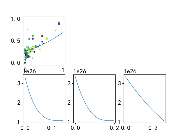
第一次体会到了,人工智能中的调参,一直调迭代的次数,然后看a,b,c三个参数的收敛情况,然后来调学习率
学习率过大的情况
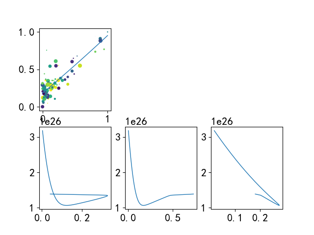
学习率过小的情况
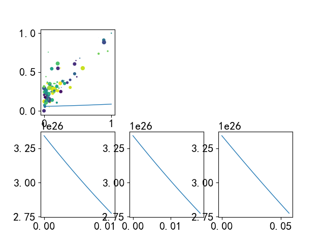
合适
代码与数据
main.py
"""
    @Time    : 2022/8/6 19:23
    @Author  : Hoppz
    @File    : 单变量高次函数拟合.py
    @Description : 数据 y = ax^2 + b 这个函数
"""
import math, copy
import numpy as np
import matplotlib.pyplot as plt
import hoppz_plt_util
from matplotlib.colors import LogNorm
from mpl_toolkits.mplot3d import axes3d, Axes3D
import pandas as pd

x_train = np.array([1, 3.0])
y_train = np.array([6.0, 8.0])

# 计算 y = ax^2 + bx + c
def compute_model_output(x,a,b,c):
    m = x.shape[0]

    f_abc = np.zeros(m)
    for i in range (m):
        f_abc[i] = a * (x**2) + b * x[i] + c

    return f_abc

# 计算均方误差
def compute_cost(x,y,a,b,c):
    m = x.shape[0]

    cost_sum = 0
    for i in range(m):
        f_abc = a * (x[i]**2) + b * x[i] + c

        cost = (f_abc - y[i]) ** 2
        cost_sum = cost_sum + cost_sum + cost
    total_cost = (1/(2 * m)) * cost_sum

    return total_cost


#  梯度计算
def compute_gradient(x,y,a,b,c):
    m = x.shape[0]

    dj_da = 0
    dj_db = 0
    dj_dc = 0
    for i in range(m):
        f_abc = a * (x[i]**2) + b * x[i] + c
        dj_da_i = (f_abc - y[i]) * (x[i]**2)
        dj_db_i = (f_abc - y[i]) * (x[i])
        dj_dc_i = (f_abc - y[i])
        dj_da = dj_da + dj_da_i
        dj_db = dj_db + dj_db_i
        dj_dc = dj_dc + dj_dc_i
    dj_da = dj_da / m
    dj_db = dj_db / m
    dj_dc = dj_dc / m

    return dj_da,dj_db,dj_dc

# 梯度下降算法
def gradient_descent(x,y,a_in,b_in,c_in,alpha, num_iters, cost_function, gradient_function):

    # 便于之后画图,记录每次迭代的数据
    # J: 本次均方误差的值
    # p: 记录迭代后 w,b 的值
    J_history = []
    p_history = []
    portray_history = []
    a = a_in
    b = b_in
    c = c_in

    # 迭代 num_iters 次
    for i in range(num_iters):
        # 计算当前 w, b 情况下的偏导数
        dj_da, dj_db, dj_dc = gradient_function(x, y, a, b, c)

        # 由损失函数的返回值来更新 w,b
        a = a - alpha * dj_da
        b = b - alpha * dj_db
        c = c - alpha * dj_dc
        # 记录每次迭代的结果
        if i < 100000:
            J_history.append(cost_function(x, y, a, b, c))
            p_history.append([a, b, c])

        # 打印当前迭代结果
        if i % math.ceil(num_iters / 10) == 0:
            portray_history.append([a, b, c])
            print(f"Iterator {i:4}:Cost {J_history[-1]:0.2e}",
                  f"dj_da: {dj_da: 0.3e}, dj_db: {dj_db: 0.3e} , dj_dc: {dj_dc: 0.3e}  ",
                  f"a: {a: 0.3e}, b:{b: 0.5e}, c:{c: 0.5e}")

    return a, b, c, J_history, p_history, portray_history
# 读入数据并存入 Numpy 数组中
def loadTxtData():
    # ---绘图设置参数---
    font = {
        'family': 'SimHei',
        'weight': 'bold',
        'size': '16'
    }
    plt.rc('font', **font)
    plt.rc('axes', unicode_minus=False)

    data_loc = "D:\workProgram\PaperSpace\gesture\PythonCode\work\single_data.txt"
    na = np.loadtxt(data_loc)
    print(f"shape is {na.shape}")
    global x_train, y_train
    x_train = na[:, 0]
    y_train = na[:, 1]

#  对数据进行归一化处理
def normalize(x):
    tx = x.copy()
    num_max = tx.max()
    num_min = tx.min()
    print(f'min : {num_min}')
    print(f'max : {num_max}')
    m = x.shape[0]

    for i in range(m):
        tx[i] = (x[i] - num_min) / (num_max - num_min)
    return tx


def doTrain():
    # ------梯度下降算法
    a_init = 0
    b_init = 0
    c_init = 0
    # some gradient descent settings
    iterations = 150000
    tmp_alpha = 5.0e-5  # 0.001

    # 归一化
    global x_train,y_train
    x_train = normalize(x_train)
    y_train = normalize(y_train)

    a_final, b_final,c_final, J_hist, p_hist, portray = gradient_descent(x_train, y_train, a_init, b_init,c_init, tmp_alpha,
                                                                 iterations, compute_cost, compute_gradient)
    print(f"(a,b,c) found by gradient descent: ({a_final:8.4f},{b_final:8.4f},{c_final:8.4f})")
    p_hist = np.array(p_hist) # 如果不转换无法用切片访问第一列的所有元素
    ##
    plt.subplot(2,3,1)
    x = np.linspace(0, 1, 50)
    y = a_final * (x**2) + b_final * x + c_final
    hoppz_plt_util.single_scatter(x_train, y_train, "size of house", "price of house")
    hoppz_plt_util.draw_line_abc(x,y , "the predict model")
    ##
    plt.subplot(2,3,4)
    hoppz_plt_util.draw_line_abc(p_hist[:,0], J_hist, "the predict model")
    plt.subplot(2,3,5)
    hoppz_plt_util.draw_line_abc(p_hist[:, 1], J_hist, "the predict model")
    plt.subplot(2,3,6)
    hoppz_plt_util.draw_line_abc(p_hist[:, 2], J_hist, "the predict model")
    plt.show()


if __name__ == '__main__':

    loadTxtData()
    doTrain()
hoppz_plt_util.py 绘制图像的自定义包
import math, copy
import numpy as np
import matplotlib.pyplot as plt
from matplotlib.colors import LogNorm
from mpl_toolkits.mplot3d import axes3d, Axes3D

plt.rcParams['font.sans-serif']=['SimHei']  # 用来正常显示中文标签
plt.rcParams['axes.unicode_minus']=False     # 用来正常显示负号

# fmt = '[marker][line][color]'
"""
    # marker ( portray point )
        '.' : 实心原点  'o' : 实心圆   '^' : 上三角   's' : 正方形
        'p' : 五边形   '*' : 星号    '+' : 加号    '...'
    # color ( the color of line )
        'r' : red   'g' : green     'b' : blue      'c' : 青色
        'm' : 品红    'y' : yellow    'k' : black     'w' : white
    # style ( the style of line )
        '-' : 实线    ':' : 虚线    '-.' : 点划线    '--' : 破折线
    # size of marker
        'ms' : marker size
        'mf' : marker face color , the inner color of point
        'mec' : marker edge color ,the border color of point
"""

# 默认设置


# 单元散点图
def single_scatter(x,y,x_label,y_label):
    np.random.seed(19680801)

    N = x.shape[0]
    colors = np.random.rand(N)
    area = (5 * np.random.rand(x.shape[0])) ** 2
    # alpha 透明度
    plt.scatter(x, y, s=area, c=colors, alpha=1)

# 画线
def draw_line_wb(x,w,b,line_lable):
    plt.plot(x,w*x+b,linewidth=1)

# 一元二次方程
def draw_line_abc(x,y,line_lable):
    plt.plot(x,y,linewidth=1)
single_data.txt
6.1101 17.592
5.5277 9.1302
8.5186 13.662
7.0032 11.854
5.8598 6.8233
8.3829 11.886
7.4764 4.3483
8.5781 12
6.4862 6.5987
5.0546 3.8166
5.7107 3.2522
14.164 15.505
5.734 3.1551
8.4084 7.2258
5.6407 0.71618
5.3794 3.5129
6.3654 5.3048
5.1301 0.56077
6.4296 3.6518
7.0708 5.3893
6.1891 3.1386
20.27 21.767
5.4901 4.263
6.3261 5.1875
5.5649 3.0825
18.945 22.638
12.828 13.501
10.957 7.0467
13.176 14.692
22.203 24.147
5.2524 -1.22
6.5894 5.9966
9.2482 12.134
5.8918 1.8495
8.2111 6.5426
7.9334 4.5623
8.0959 4.1164
5.6063 3.3928
12.836 10.117
6.3534 5.4974
5.4069 0.55657
6.8825 3.9115
11.708 5.3854
5.7737 2.4406
7.8247 6.7318
7.0931 1.0463
5.0702 5.1337
5.8014 1.844
11.7 8.0043
5.5416 1.0179
7.5402 6.7504
5.3077 1.8396
7.4239 4.2885
7.6031 4.9981
6.3328 1.4233
6.3589 -1.4211
6.2742 2.4756
5.6397 4.6042
9.3102 3.9624
9.4536 5.4141
8.8254 5.1694
5.1793 -0.74279
21.279 17.929
14.908 12.054
18.959 17.054
7.2182 4.8852
8.2951 5.7442
10.236 7.7754
5.4994 1.0173
20.341 20.992
10.136 6.6799
7.3345 4.0259
6.0062 1.2784
7.2259 3.3411
5.0269 -2.6807
6.5479 0.29678
7.5386 3.8845
5.0365 5.7014
10.274 6.7526
5.1077 2.0576
5.7292 0.47953
5.1884 0.20421
6.3557 0.67861
9.7687 7.5435
6.5159 5.3436
8.5172 4.2415
9.1802 6.7981
6.002 0.92695
5.5204 0.152
5.0594 2.8214
5.7077 1.8451
7.6366 4.2959
5.8707 7.2029
5.3054 1.9869
8.2934 0.14454
13.394 9.0551
5.4369 0.61705

 浙公网安备 33010602011771号