第1章 Pandas基础

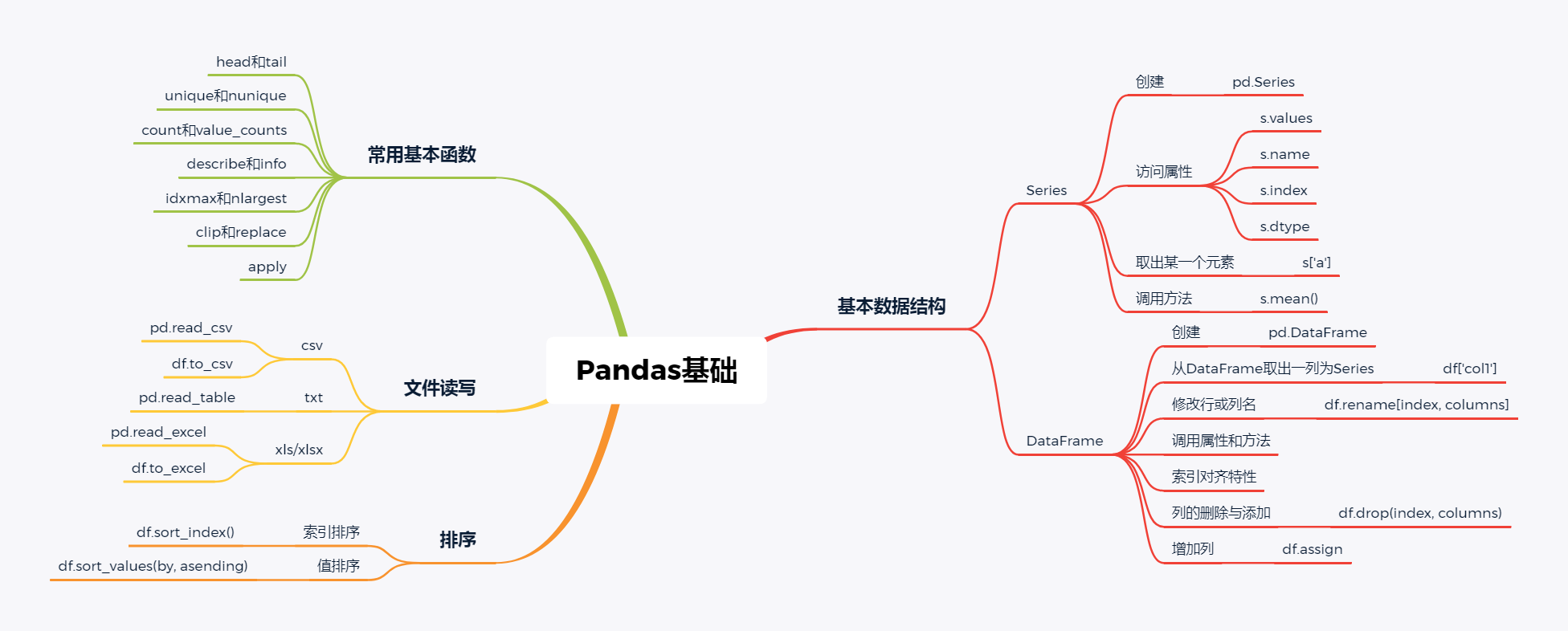
第1章 Pandas基础

import pandas as pd
import numpy as np

查看Pandas版本

pd.__version__

'1.0.3'

一、文件读取与写入

1. 读取

（a）csv格式

df = pd.read_csv('data/table.csv')
df.head()

	School	Class	ID	Gender	Address	Height	Weight	Math	Physics
0	S_1	C_1	1101	M	street_1	173	63	34.0	A+
1	S_1	C_1	1102	F	street_2	192	73	32.5	B+
2	S_1	C_1	1103	M	street_2	186	82	87.2	B+
3	S_1	C_1	1104	F	street_2	167	81	80.4	B-
4	S_1	C_1	1105	F	street_4	159	64	84.8	B+

（b）txt格式

df_txt = pd.read_table('data/table.txt') #可设置sep分隔符参数
df_txt

	col1	col2	col3	col4
0	2	a	1.4	apple
1	3	b	3.4	banana
2	6	c	2.5	orange
3	5	d	3.2	lemon

（c）xls或xlsx格式

#需要安装xlrd包
df_excel = pd.read_excel('data/table.xlsx')
df_excel.head()

	School	Class	ID	Gender	Address	Height	Weight	Math	Physics
0	S_1	C_1	1101	M	street_1	173	63	34.0	A+
1	S_1	C_1	1102	F	street_2	192	73	32.5	B+
2	S_1	C_1	1103	M	street_2	186	82	87.2	B+
3	S_1	C_1	1104	F	street_2	167	81	80.4	B-
4	S_1	C_1	1105	F	street_4	159	64	84.8	B+

2. 写入

（a）csv格式

df.to_csv('data/new_table.csv')
#df.to_csv('data/new_table.csv', index=False) #保存时除去行索引

（b）xls或xlsx格式

#需要安装openpyxl
df.to_excel('data/new_table2.xlsx', sheet_name='Sheet1')

二、基本数据结构

1. Series

（a）创建一个Series

对于一个Series，其中最常用的属性为值（values），索引（index），名字（name），类型（dtype）

s = pd.Series(np.random.randn(5),index=['a','b','c','d','e'],name='这是一个Series',dtype='float64')
s

a -0.152799
b -1.208334
c 0.668842
d 1.547519
e 0.309276
Name: 这是一个Series, dtype: float64

（b）访问Series属性

s.values

array([-0.15279875, -1.20833379, 0.6688421 , 1.54751933, 0.30927643])

s.name

'这是一个Series'

s.index

Index(['a', 'b', 'c', 'd', 'e'], dtype='object')

s.dtype

dtype('float64')

（c）取出某一个元素

将在第2章详细讨论索引的应用，这里先大致了解

s['a']

-0.15279874545981778

（d）调用方法

s.mean()

0.23290106551625706

Series有相当多的方法可以调用：

print([attr for attr in dir(s) if not attr.startswith('_')])

['T', 'a', 'abs', 'add', 'add_prefix', 'add_suffix', 'agg', 'aggregate', 'align', 'all', 'any', 'append', 'apply', 'argmax', 'argmin', 'argsort', 'array', 'asfreq', 'asof', 'astype', 'at', 'at_time', 'attrs', 'autocorr', 'axes', 'b', 'between', 'between_time', 'bfill', 'bool', 'c', 'clip', 'combine', 'combine_first', 'convert_dtypes', 'copy', 'corr', 'count', 'cov', 'cummax', 'cummin', 'cumprod', 'cumsum', 'd', 'describe', 'diff', 'div', 'divide', 'divmod', 'dot', 'drop', 'drop_duplicates', 'droplevel', 'dropna', 'dtype', 'dtypes', 'duplicated', 'e', 'empty', 'eq', 'equals', 'ewm', 'expanding', 'explode', 'factorize', 'ffill', 'fillna', 'filter', 'first', 'first_valid_index', 'floordiv', 'ge', 'get', 'groupby', 'gt', 'hasnans', 'head', 'hist', 'iat', 'idxmax', 'idxmin', 'iloc', 'index', 'infer_objects', 'interpolate', 'is_monotonic', 'is_monotonic_decreasing', 'is_monotonic_increasing', 'is_unique', 'isin', 'isna', 'isnull', 'item', 'items', 'iteritems', 'keys', 'kurt', 'kurtosis', 'last', 'last_valid_index', 'le', 'loc', 'lt', 'mad', 'map', 'mask', 'max', 'mean', 'median', 'memory_usage', 'min', 'mod', 'mode', 'mul', 'multiply', 'name', 'nbytes', 'ndim', 'ne', 'nlargest', 'notna', 'notnull', 'nsmallest', 'nunique', 'pct_change', 'pipe', 'plot', 'pop', 'pow', 'prod', 'product', 'quantile', 'radd', 'rank', 'ravel', 'rdiv', 'rdivmod', 'reindex', 'reindex_like', 'rename', 'rename_axis', 'reorder_levels', 'repeat', 'replace', 'resample', 'reset_index', 'rfloordiv', 'rmod', 'rmul', 'rolling', 'round', 'rpow', 'rsub', 'rtruediv', 'sample', 'searchsorted', 'sem', 'set_axis', 'shape', 'shift', 'size', 'skew', 'slice_shift', 'sort_index', 'sort_values', 'squeeze', 'std', 'sub', 'subtract', 'sum', 'swapaxes', 'swaplevel', 'tail', 'take', 'to_clipboard', 'to_csv', 'to_dict', 'to_excel', 'to_frame', 'to_hdf', 'to_json', 'to_latex', 'to_list', 'to_markdown', 'to_numpy', 'to_period', 'to_pickle', 'to_sql', 'to_string', 'to_timestamp', 'to_xarray', 'transform', 'transpose', 'truediv', 'truncate', 'tshift', 'tz_convert', 'tz_localize', 'unique', 'unstack', 'update', 'value_counts', 'values', 'var', 'view', 'where', 'xs']

2. DataFrame

（a）创建一个DataFrame

df = pd.DataFrame({'col1':list('abcde'),'col2':range(5,10),'col3':[1.3,2.5,3.6,4.6,5.8]},
                 index=list('一二三四五'))
df

	col1	col2	col3
一	a	5	1.3
二	b	6	2.5
三	c	7	3.6
四	d	8	4.6
五	e	9	5.8

（b）从DataFrame取出一列为Series

df['col1']

一 a
二 b
三 c
四 d
五 e
Name: col1, dtype: object

type(df)

pandas.core.frame.DataFrame

type(df['col1'])

pandas.core.series.Series

（c）修改行或列名

df.rename(index={'一':'one'},columns={'col1':'new_col1'})

	new_col1	col2	col3
one	a	5	1.3
二	b	6	2.5
三	c	7	3.6
四	d	8	4.6
五	e	9	5.8

（d）调用属性和方法

df.index

Index(['一', '二', '三', '四', '五'], dtype='object')

df.columns

Index(['col1', 'col2', 'col3'], dtype='object')

df.values

array([['a', 5, 1.3],
['b', 6, 2.5],
['c', 7, 3.6],
['d', 8, 4.6],
['e', 9, 5.8]], dtype=object)

df.shape

(5, 3)

df.mean() #本质上是一种Aggregation操作，将在第3章详细介绍

col2 7.00
col3 3.56
dtype: float64

（e）索引对齐特性

这是Pandas中非常强大的特性，不理解这一特性有时就会造成一些麻烦

df1 = pd.DataFrame({'A':[1,2,3]},index=[1,2,3])
df2 = pd.DataFrame({'A':[1,2,3]},index=[3,1,2])
df1-df2 #由于索引对齐，因此结果不是0

	A
1	-1
2	-1
3	2

（f）列的删除与添加

对于删除而言，可以使用drop函数或del或pop

df.drop(index='五',columns='col1') #设置inplace=True后会直接在原DataFrame中改动

	col2	col3
一	5	1.3
二	6	2.5
三	7	3.6
四	8	4.6

df['col1']=[1,2,3,4,5]
del df['col1']
df

	col2	col3
一	5	1.3
二	6	2.5
三	7	3.6
四	8	4.6
五	9	5.8

pop方法直接在原来的DataFrame上操作，且返回被删除的列，与python中的pop函数类似

df['col1']=[1,2,3,4,5]
df.pop('col1')

一 1
二 2
三 3
四 4
五 5
Name: col1, dtype: int64

df

	col2	col3
一	5	1.3
二	6	2.5
三	7	3.6
四	8	4.6
五	9	5.8

可以直接增加新的列，也可以使用assign方法

df1['B']=list('abc')
df1

	A	B
1	1	a
2	2	b
3	3	c

df1.assign(C=pd.Series(list('def')))
#思考：为什么会出现NaN？（提示：索引对齐）assign左右两边的索引不一样，请问结果的索引谁说了算？

	A	B	C
1	1	a	e
2	2	b	f
3	3	c	NaN

但assign方法不会对原DataFrame做修改

df1

	A	B
1	1	a
2	2	b
3	3	c

（g）根据类型选择列

df.select_dtypes(include=['number']).head()

	col2	col3
一	5	1.3
二	6	2.5
三	7	3.6
四	8	4.6
五	9	5.8

df.select_dtypes(include=['float']).head()

	col3
一	1.3
二	2.5
三	3.6
四	4.6
五	5.8

（h）将Series转换为DataFrame

s = df.mean()
s.name='to_DataFrame'
s

col2 7.00
col3 3.56
Name: to_DataFrame, dtype: float64

s.to_frame()

	to_DataFrame
col2	7.00
col3	3.56

使用T符号可以转置

s.to_frame().T

	col2	col3
to_DataFrame	7.0	3.56

三、常用基本函数

从下面开始，包括后面所有章节，我们都会用到这份虚拟的数据集

df = pd.read_csv('data/table.csv')

1. head和tail

df.head()

	School	Class	ID	Gender	Address	Height	Weight	Math	Physics
0	S_1	C_1	1101	M	street_1	173	63	34.0	A+
1	S_1	C_1	1102	F	street_2	192	73	32.5	B+
2	S_1	C_1	1103	M	street_2	186	82	87.2	B+
3	S_1	C_1	1104	F	street_2	167	81	80.4	B-
4	S_1	C_1	1105	F	street_4	159	64	84.8	B+

df.tail()

	School	Class	ID	Gender	Address	Height	Weight	Math	Physics
30	S_2	C_4	2401	F	street_2	192	62	45.3	A
31	S_2	C_4	2402	M	street_7	166	82	48.7	B
32	S_2	C_4	2403	F	street_6	158	60	59.7	B+
33	S_2	C_4	2404	F	street_2	160	84	67.7	B
34	S_2	C_4	2405	F	street_6	193	54	47.6	B

可以指定n参数显示多少行

df.head(3)

	School	Class	ID	Gender	Address	Height	Weight	Math	Physics
0	S_1	C_1	1101	M	street_1	173	63	34.0	A+
1	S_1	C_1	1102	F	street_2	192	73	32.5	B+
2	S_1	C_1	1103	M	street_2	186	82	87.2	B+

2. unique和nunique

nunique显示有多少个唯一值

df['Physics'].nunique()

7

unique显示所有的唯一值

df['Physics'].unique()

array(['A+', 'B+', 'B-', 'A-', 'B', 'A', 'C'], dtype=object)

3. count和value_counts

count返回非缺失值元素个数

df['Physics'].count()

35

value_counts返回每个元素有多少个

df['Physics'].value_counts()

B+ 9
B 8
B- 6
A 4
A+ 3
A- 3
C 2
Name: Physics, dtype: int64

4. describe和info

info函数返回有哪些列、有多少非缺失值、每列的类型

df.info()

<class 'pandas.core.frame.DataFrame'>
RangeIndex: 35 entries, 0 to 34
Data columns (total 9 columns):
# Column Non-Null Count Dtype
--- ------ -------------- -----
0 School 35 non-null object
1 Class 35 non-null object
2 ID 35 non-null int64
3 Gender 35 non-null object
4 Address 35 non-null object
5 Height 35 non-null int64
6 Weight 35 non-null int64
7 Math 35 non-null float64
8 Physics 35 non-null object
dtypes: float64(1), int64(3), object(5)
memory usage: 2.6+ KB

describe默认统计数值型数据的各个统计量

df.describe()

	ID	Height	Weight	Math
count	35.00000	35.000000	35.000000	35.000000
mean	1803.00000	174.142857	74.657143	61.351429
std	536.87741	13.541098	12.895377	19.915164
min	1101.00000	155.000000	53.000000	31.500000
25%	1204.50000	161.000000	63.000000	47.400000
50%	2103.00000	173.000000	74.000000	61.700000
75%	2301.50000	187.500000	82.000000	77.100000
max	2405.00000	195.000000	100.000000	97.000000

可以自行选择分位数

df.describe(percentiles=[.05, .25, .75, .95])

	ID	Height	Weight	Math
count	35.00000	35.000000	35.000000	35.000000
mean	1803.00000	174.142857	74.657143	61.351429
std	536.87741	13.541098	12.895377	19.915164
min	1101.00000	155.000000	53.000000	31.500000
5%	1102.70000	157.000000	56.100000	32.640000
25%	1204.50000	161.000000	63.000000	47.400000
50%	2103.00000	173.000000	74.000000	61.700000
75%	2301.50000	187.500000	82.000000	77.100000
95%	2403.30000	193.300000	97.600000	90.040000
max	2405.00000	195.000000	100.000000	97.000000

对于非数值型也可以用describe函数

df['Physics'].describe()

count 35
unique 7
top B+
freq 9
Name: Physics, dtype: object

5. idxmax和nlargest

idxmax函数返回最大值所在索引，在某些情况下特别适用，idxmin功能类似

df['Math'].idxmax()

5

nlargest函数返回前几个大的元素值，nsmallest功能类似

df['Math'].nlargest(3)

5 97.0
28 95.5
11 87.7
Name: Math, dtype: float64

6. clip和replace

clip和replace是两类替换函数

clip是对超过或者低于某些值的数进行截断

df['Math'].head()

0 34.0
1 32.5
2 87.2
3 80.4
4 84.8
Name: Math, dtype: float64

df['Math'].clip(33,80).head()

0 34.0
1 33.0
2 80.0
3 80.0
4 80.0
Name: Math, dtype: float64

df['Math'].mad() 

16.924244897959188

replace是对某些值进行替换

df['Address'].head()

0 street_1
1 street_2
2 street_2
3 street_2
4 street_4
Name: Address, dtype: object

df['Address'].replace(['street_1','street_2'],['one','two']).head()

0 one
1 two
2 two
3 two
4 street_4
Name: Address, dtype: object

通过字典，可以直接在表中修改

df.replace({'Address':{'street_1':'one','street_2':'two'}}).head()

	School	Class	ID	Gender	Address	Height	Weight	Math	Physics
0	S_1	C_1	1101	M	one	173	63	34.0	A+
1	S_1	C_1	1102	F	two	192	73	32.5	B+
2	S_1	C_1	1103	M	two	186	82	87.2	B+
3	S_1	C_1	1104	F	two	167	81	80.4	B-
4	S_1	C_1	1105	F	street_4	159	64	84.8	B+

7. apply函数

apply是一个自由度很高的函数，在第3章我们还要提到

对于Series，它可以迭代每一列的值操作：

df['Math'].apply(lambda x:str(x)+'!').head() #可以使用lambda表达式，也可以使用函数

0 34.0!
1 32.5!
2 87.2!
3 80.4!
4 84.8!
Name: Math, dtype: object

对于DataFrame，它在默认axis=0下可以迭代每一个列操作：

df.apply(lambda x:x.apply(lambda x:str(x)+'!')).head() #这是一个稍显复杂的例子，有利于理解apply的功能

	School	Class	ID	Gender	Address	Height	Weight	Math	Physics
0	S_1!	C_1!	1101!	M!	street_1!	173!	63!	34.0!	A+!
1	S_1!	C_1!	1102!	F!	street_2!	192!	73!	32.5!	B+!
2	S_1!	C_1!	1103!	M!	street_2!	186!	82!	87.2!	B+!
3	S_1!	C_1!	1104!	F!	street_2!	167!	81!	80.4!	B-!
4	S_1!	C_1!	1105!	F!	street_4!	159!	64!	84.8!	B+!

Pandas中的axis参数=0时，永远表示的是处理方向而不是聚合方向，当axis='index'或=0时，对列迭代对行聚合，行即为跨列，axis=1同理

四、排序

1. 索引排序

df.set_index('Math').head() #set_index函数可以设置索引，将在下一章详细介绍

	School	Class	ID	Gender	Address	Height	Weight	Physics
Math
34.0	S_1	C_1	1101	M	street_1	173	63	A+
32.5	S_1	C_1	1102	F	street_2	192	73	B+
87.2	S_1	C_1	1103	M	street_2	186	82	B+
80.4	S_1	C_1	1104	F	street_2	167	81	B-
84.8	S_1	C_1	1105	F	street_4	159	64	B+

df.set_index('Math').sort_index().head() #可以设置ascending参数，默认为升序，True

	School	Class	ID	Gender	Address	Height	Weight	Physics
Math
31.5	S_1	C_3	1301	M	street_4	161	68	B+
32.5	S_1	C_1	1102	F	street_2	192	73	B+
32.7	S_2	C_3	2302	M	street_5	171	88	A
33.8	S_1	C_2	1204	F	street_5	162	63	B
34.0	S_1	C_1	1101	M	street_1	173	63	A+

2. 值排序

df.sort_values(by='Class').head()

	School	Class	ID	Gender	Address	Height	Weight	Math	Physics
0	S_1	C_1	1101	M	street_1	173	63	34.0	A+
19	S_2	C_1	2105	M	street_4	170	81	34.2	A
18	S_2	C_1	2104	F	street_5	159	97	72.2	B+
16	S_2	C_1	2102	F	street_6	161	61	50.6	B+
15	S_2	C_1	2101	M	street_7	174	84	83.3	C

多个值排序，即先对第一层排，在第一层相同的情况下对第二层排序

df.sort_values(by=['Address','Height']).head()

	School	Class	ID	Gender	Address	Height	Weight	Math	Physics
0	S_1	C_1	1101	M	street_1	173	63	34.0	A+
11	S_1	C_3	1302	F	street_1	175	57	87.7	A-
23	S_2	C_2	2204	M	street_1	175	74	47.2	B-
33	S_2	C_4	2404	F	street_2	160	84	67.7	B
3	S_1	C_1	1104	F	street_2	167	81	80.4	B-

五、问题与练习

1. 问题

【问题一】 Series和DataFrame有哪些常见属性和方法？

【问题二】 value_counts会统计缺失值吗？

【问题三】 如果有多个索引同时取到最大值，idxmax会返回所有这些索引吗？如果不会，那么怎么返回这些索引？

【问题四】 在常用函数一节中，由于一些函数的功能比较简单，因此没有列入，现在将它们列在下面，请分别说明它们的用途并尝试使用。

sum/mean/median/mad/min/max/abs/std/var/quantile/cummax/cumsum/cumprod

【问题五】 df.mean(axis=1)是什么意思？它与df.mean()的结果一样吗？问题四提到的函数也有axis参数吗？怎么使用？

【问题六】 对值进行排序后，相同的值次序由什么决定？

【问题七】 Pandas中为各类基础运算也定义了函数，比如s1.add(s2)表示两个Series相加，但既然已经有了'+'，是不是多此一举？

【问题八】 如果DataFrame某一列的元素是numpy数组，那么将其保存到csv在读取后就会变成字符串，怎么解决？

2. 练习

【练习一】 现有一份关于美剧《权力的游戏》剧本的数据集，请解决以下问题：

（a）在所有的数据中，一共出现了多少人物？

（b）以单元格计数（即简单把一个单元格视作一句），谁说了最多的话？

（c）以单词计数，谁说了最多的单词？（不是单句单词最多，是指每人说过单词的总数最多，为了简便，只以空格为单词分界点，不考虑其他情况）

pd.read_csv('data/Game_of_Thrones_Script.csv').head()

	Release Date	Season	Episode	Episode Title	Name	Sentence
0	2011/4/17	Season 1	Episode 1	Winter is Coming	waymar royce	What do you expect? They're savages. One lot s...
1	2011/4/17	Season 1	Episode 1	Winter is Coming	will	I've never seen wildlings do a thing like this...
2	2011/4/17	Season 1	Episode 1	Winter is Coming	waymar royce	How close did you get?
3	2011/4/17	Season 1	Episode 1	Winter is Coming	will	Close as any man would.
4	2011/4/17	Season 1	Episode 1	Winter is Coming	gared	We should head back to the wall.

【练习二】现有一份关于科比的投篮数据集，请解决如下问题：

（a）哪种action_type和combined_shot_type的组合是最多的？

（b）在所有被记录的game_id中，遭遇到最多的opponent是一个支？（由于一场比赛会有许多次投篮，但对阵的对手只有一个，本题相当 于问科比和哪个队交锋次数最多）

pd.read_csv('data/Kobe_data.csv',index_col='shot_id').head()
#index_col的作用是将某一列作为行索引

	action_type	combined_shot_type	game_event_id	game_id	lat	loc_x	loc_y	lon	minutes_remaining	period	...	shot_made_flag	shot_type	shot_zone_area	shot_zone_basic	shot_zone_range	team_id	team_name	game_date	matchup	opponent
shot_id
1	Jump Shot	Jump Shot	10	20000012	33.9723	167	72	-118.1028	10	1	...	NaN	2PT Field Goal	Right Side(R)	Mid-Range	16-24 ft.	1610612747	Los Angeles Lakers	2000/10/31	LAL @ POR	POR
2	Jump Shot	Jump Shot	12	20000012	34.0443	-157	0	-118.4268	10	1	...	0.0	2PT Field Goal	Left Side(L)	Mid-Range	8-16 ft.	1610612747	Los Angeles Lakers	2000/10/31	LAL @ POR	POR
3	Jump Shot	Jump Shot	35	20000012	33.9093	-101	135	-118.3708	7	1	...	1.0	2PT Field Goal	Left Side Center(LC)	Mid-Range	16-24 ft.	1610612747	Los Angeles Lakers	2000/10/31	LAL @ POR	POR
4	Jump Shot	Jump Shot	43	20000012	33.8693	138	175	-118.1318	6	1	...	0.0	2PT Field Goal	Right Side Center(RC)	Mid-Range	16-24 ft.	1610612747	Los Angeles Lakers	2000/10/31	LAL @ POR	POR
5	Driving Dunk Shot	Dunk	155	20000012	34.0443	0	0	-118.2698	6	2	...	1.0	2PT Field Goal	Center(C)	Restricted Area	Less Than 8 ft.	1610612747	Los Angeles Lakers	2000/10/31	LAL @ POR	POR

5 rows × 24 columns