

一、学习资料:
北京博雅数据酷客平台大讲堂:http://cookdata.cn/auditorium/course_room/10015/
案例连接:http://cookdata.cn/note/view_static_note/61f373ccecf93d7ecb7fd03e11e7ff3e/
二、分布梳理
分类决策树Python实现
1、定义决策树节点
2、基尼系数计算
3、分类决策树生成
4、使用Networkx将决策树可视化
5、决策树的决策边界
6、实现决策树的预测函数
三、代码实现
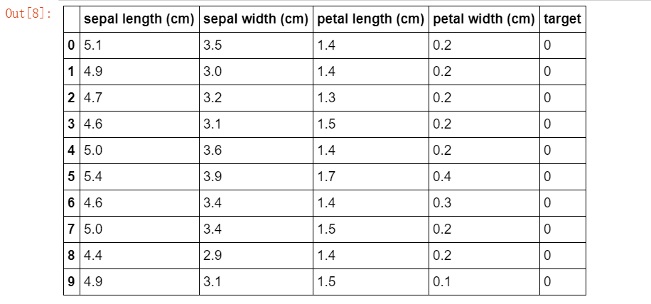
首先加载一份鸢尾花数据用于测试,在Sklearn中可以使用datasets.load_iris方法直接加载数据集。鸢尾花数据集包含150个鸢尾花样本,每个样本包含四个特征和一个类别标签。
from sklearn.datasets import load_iris
import pandas as pd
iris=load_iris()
iris_df=pd.DataFrame(data=iris.data,columns=iris.feature_names)
iris_df["target"]=iris.target
iris_df.head()
iris_df.columxs=["sepal_len","sepal_width","petal_len","petal_width","target"]
X_iris=iris_df.iloc[:,:-1]
y_iris=iris_df["target"]
iris_df.head(10) #显示默认行数
1、定义决策树节点。创建一个表示决策树节点的类TreeNode。决策树节点需要存储的最重要的信息为当前节点代表的特征。如果节点是非叶子节点,还需要存储做儿子节点left和右儿子节点right。
class TreeNode:
    def _init_(self,x_pos,y_pos,layer,class_labels=[0,1,2]):
        self.f=None #当前节点的切分特征
        self.v=None #当前节点的切分点
        self.left=None #左儿子节点
        self.right=None #右儿子节点
        self.pos=(x_pos,y_pos)#节点坐标,进行可视化
        self.label_dist=None #当前节点样本的类分布
        self.layer=layer
        self.class_labels=class_labels
    def _str_(self):#打印节点信息,可视化时的节点标签
        if self.f!=None:
            return self.f+"\n<="+str(round(self.v,2))
        else:
            return str(self.label_dist)+"\n("+str(np.sum(self.label_dist))+")"
2、基尼系数计算
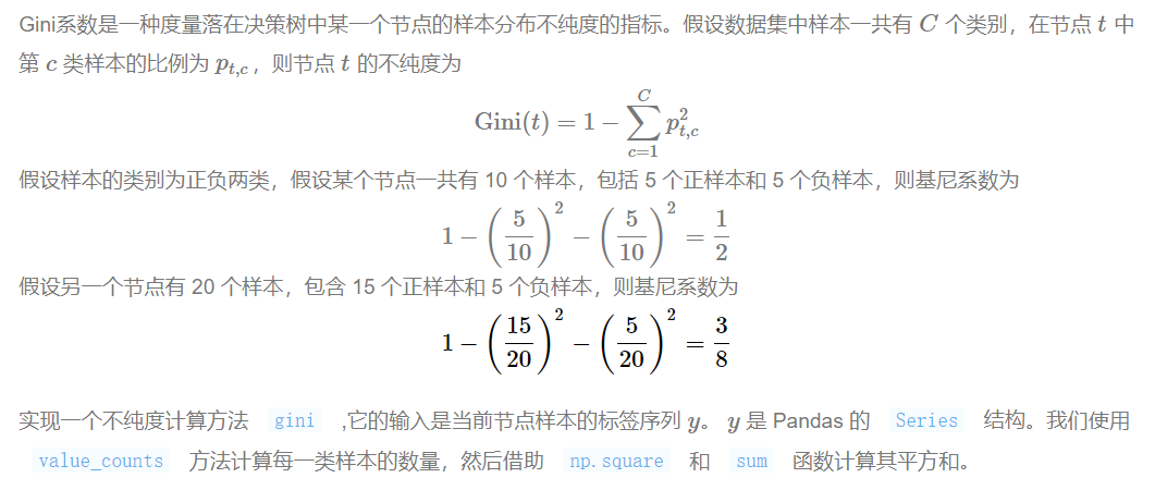
import numpy as np
def gini(y):
    #输入标签序列,返回基尼系数
    return 1-np.square(y.value_counts()/len(y)).sum()
3、分类决策树生成
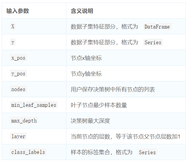
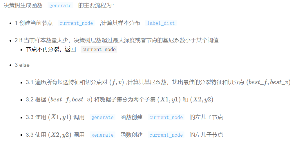
def generate(X,y,x_pos,y_pos,nodes,min_leaf_samples,max_depth,layer,class_labels):
    current_node = TreeNode(x_pos,y_pos,layer,class_labels)#创建节点对象
    current_node.label_dist = [len(y[y==v]) for v in class_labels] #当前节点类样本分布
    nodes.append(current_node)
    if(len(X) < min_leaf_samples or gini(y) < 0.1 or layer > max_depth): #判断是否需要生成子节点
        return current_node
    max_gini,best_f,best_v = 0,None,None
    for f in X.columns: #特征遍历
        for v in X[f].unique(): #取值遍历
            y1,y2 = y[X[f] <= v],y[X[f] > v]
            if (len(y1) >= min_leaf_samples and len(y2) >= min_leaf_samples):
                imp_descent =  gini(y)-gini(y1)*len(y1)/len(y)-gini(y2)*len(y2)/len(y) #****计算不纯度变化****#
                if imp_descent > max_gini:
                    max_gini,best_f,best_v = imp_descent,f,v
    current_node.f,current_node.v = best_f,best_v
    if(current_node.f != None):
        current_node.left = generate(X[X[best_f] <= best_v],y[X[best_f] <= best_v],x_pos-(2**(max_depth-layer)),y_pos -1,nodes,min_leaf_samples,max_depth,layer + 1,class_labels)
        current_node.right = generate(X[X[best_f] > best_v],y[X[best_f] > best_v],x_pos+ (2**(max_depth-layer)),y_pos -1,nodes,min_leaf_samples,max_depth,layer + 1,class_labels)
    return current_node
def decision_tree_classifier(X,y,min_leaf_samples,max_depth):
    nodes = []
    root = generate(X,y,0,0,nodes,min_leaf_samples=min_leaf_samples,max_depth=max_depth,layer=1,class_labels=y.unique())
    return root,nodes
4、使用Networkx将决策树可视化
#编写一个函数,将训练得到的决策树转换成 Networkx 中的网络对象 G
def get_networkx_graph(G, root):
    if root.left != None:
        G.add_edge(root, root.left) #在当前节点和左儿子节点之间建立一条边,加入G
        get_networkx_graph(G, root.left) #对左儿子执行同样操作
    if root.right != None:
        G.add_edge(root, root.right) #在当前节点和左儿子节点之间建立一条边,加入G
        get_networkx_graph(G,root.right)#对右儿子执行同样操作
#在决策树生成函数中,已经计算了节点的坐标。现在我们实现一个函数,输入节点集合,返回其位置布局字典对象。
def get_tree_pos(G):
    pos = {}
    for node in G.nodes:
        pos[node] = node.pos
    return pos
#在决策树中,如果是叶子节点,则根据其预测类别显示不同颜色。如果是非叶子节点,则显示灰色。
def get_node_color(G):
    color_dict = []
    for node in G.nodes:
        if node.f == None:  #叶子节点
            label = np.argmax(node.label_dist)
            if label%3 == 0:
                color_dict.append("#007979") #深绿色
            elif label%3 == 1:
                color_dict.append("#E4007F") #洋红色
            else:
                color_dict.append("blue")
        else:
            color_dict.append("gray")
    return color_dict
#在鸢尾花数据集上训练决策树,然后将学习到的决策树绘制出来。
import matplotlib.pyplot as plt
import networkx as nx
%matplotlib inline
#1训练决策树
root,nodes = decision_tree_classifier(X_iris,y_iris,min_leaf_samples=10,max_depth=4)
#2将决策树进行可视化
fig, ax = plt.subplots(figsize=(9, 9)) #2.1将图的大小设置为 9×9
graph = nx.DiGraph() #2.2 创建 Networkx 中的网络对象
get_networkx_graph(graph, root) #**** 2.3将决策树转换成 Networkx 的网络对象****#
pos = get_tree_pos(graph) #****2.4 获取节点的坐标****#
# 2.5 绘制决策树
nx.draw_networkx(graph,pos = pos,ax = ax,node_shape="o",font_color="w",node_size=5000,node_color=get_node_color(graph))
plt.box(False) #去掉边框
plt.axis("off")#不显示坐标轴
5、决策树的决策边界
import seaborn as sns
#筛选两列特征
feature_names = ["petal_len","petal_width"]
X = iris_df[feature_names]
y = iris_df["target"]
#训练决策树模型
tree_two_dimension, nodes = decision_tree_classifier(X,y,min_leaf_samples=10,max_depth=4)

fig, ax = plt.subplots(figsize=(9, 9)) #设置图片大小
sns.scatterplot(x = X.iloc[:,0], y = X.iloc[:,1],ax = ax,hue = y) #绘制样本点 scatterplot
#遍历决策树节点,绘制划分直线
for node in nodes:
    if node.f == X.columns[0]:
        ax.vlines(node.v,X.iloc[:,1].min(),X.iloc[:,1].max(),color="gray") #****如果节点分裂特征是 petal_len ,则绘制竖线****#
    elif node.f == X.columns[1]:
        ax.hlines(node.v,X.iloc[:,0].min(),X.iloc[:,0].max(),color="gray") #如果节点分裂特征是 petal_width ,则绘制水平线
6、实现决策树的预测函数
from sklearn.metrics import confusion_matrix
import seaborn as sns
import matplotlib.pyplot as plt
fig, ax = plt.subplots(figsize=(9,9))
# 设置正常显示中文
sns.set(font='SimHei')
# 绘制热力图
confusion_matrix = confusion_matrix(y_pred,iris_df["target"])#****计算混淆矩阵****#

ax = sns.heatmap(confusion_matrix,linewidths=.5,cmap="Greens",
                 annot=True, fmt='d',xticklabels=iris.target_names, yticklabels=iris.target_names)
ax.set_ylabel('真实')
ax.set_xlabel('预测')
ax.xaxis.set_label_position('top')
ax.xaxis.tick_top()
ax.set_title('混淆矩阵热力图')

