
tensorflow 2.0 学习(四)MNIST 训练与测试
这次的mnist学习加入了测试集,看看学习的准确率,代码如下
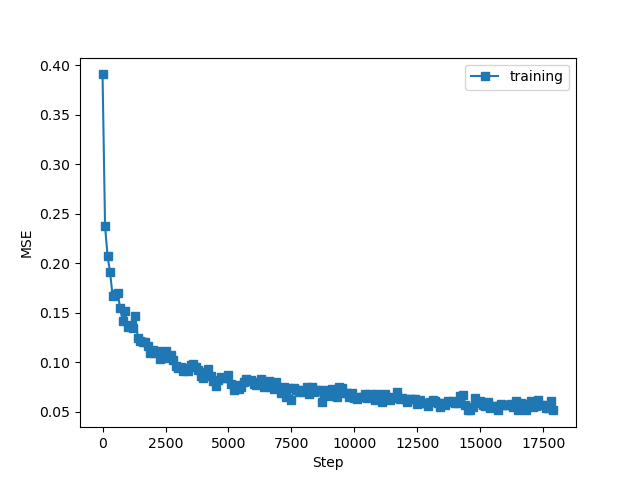
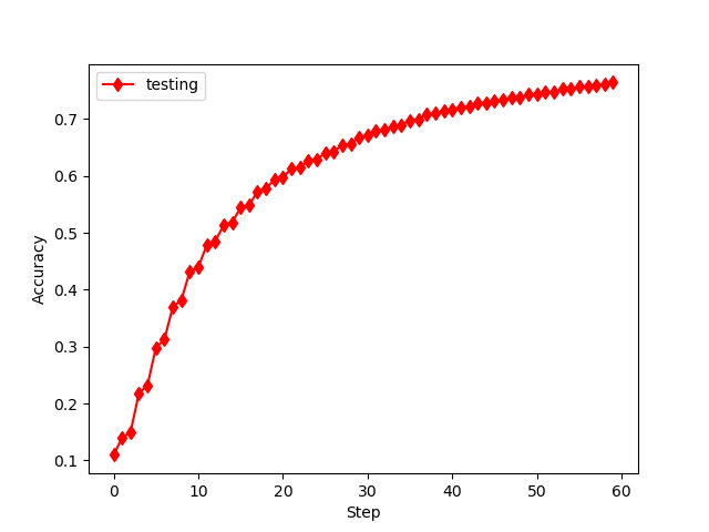
# encoding: utf-8

import tensorflow as tf
import matplotlib.pyplot as plt

#加载下载好的mnist数据库 60000张训练 10000张测试 每一张维度(28,28)
path = r'G:\2019\python\mnist.npz'
(x_train, y_train), (x_test, y_test) = tf.keras.datasets.mnist.load_data(path)

#第一层输入256, 第二次输出128, 第三层输出10
#第一,二,三层参数w,b
w1 = tf.Variable(tf.random.truncated_normal([784, 256], stddev=0.1))    #正态分布的一种
b1 = tf.Variable(tf.zeros([256]))
w2 = tf.Variable(tf.random.truncated_normal([256, 128], stddev=0.1))
b2 = tf.Variable(tf.zeros([128]))
w3 = tf.Variable(tf.random.truncated_normal([128, 10], stddev=0.1))
b3 = tf.Variable(tf.zeros([10]))

#两种数据预处理的方法
#(一)预处理训练数据
x = tf.convert_to_tensor(x_train, dtype = tf.float32)/255.    #0:1  ;   -1:1(不适合训练,准确度不高)
x = tf.reshape(x, [-1, 28*28])
y = tf.convert_to_tensor(y_train, dtype=tf.int32)
y = tf.one_hot(y, depth=10)
#将60000组训练数据切分为600组,每组100个数据
train_db = tf.data.Dataset.from_tensor_slices((x, y))
train_db = train_db.shuffle(60000)      #尽量与样本空间一样大
train_db = train_db.batch(100)          #128


#(二)自定义预处理测试函数
def preprocess(x, y):
    x = tf.cast(x, dtype=tf.float32) / 255.     #先将类型转化为float32,再归一到0-1
    x = tf.reshape(x, [-1, 28*28])              #不知道x数量,用-1代替,转化为一维784个数据
    y = tf.cast(y, dtype=tf.int32)              #转化为整型32
    y = tf.one_hot(y, depth=10)                 #训练数据所需的one-hot编码
    return x, y

#将10000组测试数据预处理
test_db = tf.data.Dataset.from_tensor_slices((x_test, y_test))
test_db = test_db.shuffle(10000)
test_db = test_db.batch(100)        #128
test_db = test_db.map(preprocess)

lr = 0.001      #学习率
losses = []     #储存每epoch的loss值,便于观察学习情况
acc = []        #准确率

for epoch in range(30):     #20
    #一次性处理100组(x, y)数据
    for step, (x, y) in enumerate(train_db):    #遍历切分好的数据step:0->599
        with tf.GradientTape() as tape:
            #向前传播第一,二,三层
            h1 = x@w1 + tf.broadcast_to(b1, [x.shape[0], 256])  #可以直接写成 +b1
            h1 = tf.nn.relu(h1)
            h2 = h1@w2 + b2
            h2 = tf.nn.relu(h2)
            out = h2@w3 + b3

            #计算mse
            loss = tf.square(y - out)
            loss = tf.reduce_mean(loss)
        #计算参数的梯度,tape.gradient为自动求导函数,loss为目标数据,目的使它越来越接近真实值
        grads = tape.gradient(loss, [w1, b1, w2, b2, w3, b3])
        #更新w,b
        w1.assign_sub(lr*grads[0])  #原地减去给定的值,实现参数的自我更新
        b1.assign_sub(lr*grads[1])
        w2.assign_sub(lr*grads[2])
        b2.assign_sub(lr*grads[3])
        w3.assign_sub(lr*grads[4])
        b3.assign_sub(lr*grads[5])
        #观察学习情况
        if step%100 == 0:
            print('训练第 ',epoch,'轮',', 第',step,'步, ','loss:', float(loss))
            losses.append(float(loss))          #将每100step后的loss情况储存起来,最后观察

        if step%500 == 0:
            total, total_correct = 0., 0.
            for x, y in test_db:
                h1 = x @ w1 + b1
                h1 = tf.nn.relu(h1)
                h2 = h1 @ w2 + b2
                h2 = tf.nn.relu(h2)
                out = h2 @ w3 + b3

                pred = tf.argmax(out, axis=1)  # 选取概率最大的类别
                y = tf.argmax(y, axis=1)  # 类似于one-hot逆编码
                correct = tf.equal(pred, y)  # 比较真实值和预测值是否相等
                total += x.shape[0]
                # 统计正确的个数
                total_correct += tf.reduce_sum(tf.cast(correct, dtype=tf.int32)).numpy()
            print('训练第 ',epoch,'轮',', 第',step,'步, ', 'Evaluate Acc:', total_correct/total)
            acc.append(total_correct/total)

#plt.subplot(121)
x1 = [i*100 for i in range(len(losses))]
plt.plot(x1, losses, marker='s', label='training')
plt.xlabel('Step')
plt.ylabel('MSE')
plt.legend()
#plt.savefig('exam_mnist_forward.png')
#plt.show()

#plt.subplot(122)
plt.figure()
x2 = [i for i in range(len(acc))]
plt.plot(x2, acc, 'r',marker='d', label='testing')
plt.xlabel('Step')
plt.ylabel('Accuracy')
plt.legend()
#plt.savefig('test_mnist_forward.png')
plt.show()
误差何准确率如下
发现和书中类似,但要注意的如下:
(1)数据预处理时,打散值选择和数据空间一样大;
(2)数据处理选择0-1之间,而不用(-1 :1),是因为后者学习效率不理想!
(3)代码还可以进行优化处理!
总的来说,代码还是容易理解,使用也更加简洁!
下一次更新,全连接网络,关于汽车油耗的预测。

 浙公网安备 33010602011771号