[搬运]Exponentials: Discrete, Real, and Imaginary

搬运自https://sites.google.com/site/butwhymath/algebra/eponentials-discrete-real-and-imaginary，这个博客一系列的文章都很好

国外的文章和教材有语言的障碍，但是没有理解的障碍；国内的文章和教材虽然没有语言的障碍，但是有理解的障碍。

有时间我会把其中比较关键的段落翻译一下，诸位共勉~

Exponentials: Discrete, Real, and Imaginary

指数函数（这里的含义主要是以自然对数的底数e为底的指数函数）：离散的，实数和虚数

The family of exponential functions (things of the form $a\cdot b^x$ ) are ubiquitous in mathematics, physics and engineering. Due to the relatively simple set of rules for manipulating such expressions, once learned they can be used almost without thinking, and often the meaning behind them is lost. Thus, instead of a rigorous approach, I will try to provide some bits of intuition, specifically focused on what makes e such a "special" number.

以e为底数的指数函数的家族在数学，物理学和工程学中无处不在。因为操作这些函数的规则相对简单，所以学过以后在实际计算的时候几乎不需要思考，因此这些操作背后的意义慢慢地就被遗忘了。这里我并不会非常严谨细致的讲解，而是希望能尽量提供一种直观上的理解，尤其是直观上理解这个特殊的数字是如何一步一步得来的

Repeated Multiplication

重复的乘法

Exponentials first arise out of a need for a shorthand for multiplication (much like multiplication itself can be seen as a generalization of a shorthand for addition). Lets say we have a number a which we've multiplied together a bunch of times to get b: $b=a\cdot a\cdot a\cdot a\cdot a\cdot a$ . Since there are 6 a's in this expression, we decide to write it $b=a^6$ . The rules of exponents learned in highschool are just a consequence of this notational choice. To see this, consider the number a⁴ and a². Since these are just short hand expressions for the product of 4 a's and 2 a's respectively, it is easy to see what the shorthand of their product should be:

指数标记的形式最开始来自于想要把一种复杂的记号形式简写的需求，比如同一个数字重复相乘10次，20次，或者更多次，如下面公式（当然也可以把乘法这种记号标记看做同一个数字多次相加的简写形式）。假设我们用同一个数字多次相乘了自己多次得到了数字b： $b=a\cdot a\cdot a\cdot a\cdot a\cdot a$ . 这里的式子中有6个a相乘，所以我们可以用指数形式表示： $b=a^6$ . 在高中学到的操作指数所应遵循的规则只不过是采用这种记号形式以后自然而然的延伸。举个例子，假设我们现在有两个数字a⁴ 和a²。因为这种表示形式是4个a相乘和2个a相乘的简写形式，所以很容易就可以看到这两个数字a⁴ 和a²相乘该如何计算：，

$a^4 \cdot a^2 = (a\cdot a\cdot a\cdot a)\cdot (a\cdot a)=(a \cdot a \cdot a \cdot a \cdot a \cdot a)=a^6=a^{(4+2)}$

And in general, multiplying a product of m successive a's and a product of n successive a's simply gives a product of m+n successive a's. In our shorthand then;

一般来说，m个a相乘与n个a相乘的积就是（m+n）个a相乘。简写形式为：

$a^m \cdot a^n = \underbrace{a \cdot .... \cdot a }_\textrm{m} \cdot \underbrace{a \cdot .... \cdot a }_\textrm{n}=\underbrace{a \cdot .... \cdot a }_\textrm{m+n}=a^{m+n}$

Which is nothing other than the standard rule for exponents. Now say that you have a number b which happens to be a product of three a's, that is b=a³. Is there a "nice" way to talk about the product of b with itself five times? If each b is composed of three a's and we have five b's multiplied in succession, then another way to phrase this is simply that we have 15 a's being multiplied together. In the exponential shorthand;

这种记号形式和由此而来的处理规则就是指数函数的标准规则。假设现在有一个数字b等于3个a相乘，那有没有一种简单的方式去描述5个b相乘得到的结果呢？每个数字b是由3个a相乘，而我们现在要计算5个b相乘，换句话说，现在有15个a相乘。用指数函数的记号形式去表达这个意思

，公式如下：

$(a^3)^5=(a\cdot a \cdot a)^5=(a\cdot a \cdot a)\cdot (a\cdot a \cdot a)\cdot (a\cdot a \cdot a)\cdot (a\cdot a \cdot a)\cdot (a\cdot a \cdot a)$

$=(a \cdot a \cdot a \cdota \cdot a \cdot a \cdota \cdot a \cdot a \cdota \cdot a \cdot a \cdota \cdot a \cdot a \cdota \cdot a \cdot a \cdot a \cdot a )=a^{15}=a^{3 \cdot 5}$

This also extends arbitrarily; (a^m)ⁿ says to take the number a and multiply it together m times, and then take that and multiply it by itself n times. Obviously n copies of a set of m objects placed side by side is just a list of things of length mn. This is then written in our exponential shorthand as

这个规则也可以随意的扩展：(a^m)ⁿ的意思就是m个a相乘，然后有n个这样的数相乘。显然，把m个a放在一块当做一堆，n个这么一堆排排放的话，就有mn个a。这种含义用指数符号去标记和描述如下：

$(a^m)^n = (\underbrace{a \cdot .... \cdot a }_\textrm{m})^n=\underbrace{(\underbrace{a \cdot .... \cdot a }_\textrm{m}) ....(\underbrace{a \cdot .... \cdot a }_\textrm{m})}_\textrm{n}=(\underbrace{a\cdot ... \cdot a}_\textrm{mn})=a^{mn}$

This idea of using exponents as a short hand for repeated multiplication has turned out to be quite useful, so lets see how it extends. As of now our preliminary definition is restricted to positive integer exponents (because it only makes sense to multiply things together an integer number of times). What about negative integers? If positive integer exponents give us a short hand for repeated multiplication, could it be possible to define negative integer exponents to be a short hand for repeated division? Much like a⁵ means "multiply a by itself five times", then a^-5 would signify dividing by a five times. This turns out to work well with the exponent rule above: say you multiply by a five times and then divide by a three times. This is obviously equivalent to only having multiplied by a twice, so in effect we would like it to be true that a⁵a^-3=a². But by our rule for dealing with this short hand, we already know that a⁵a^-3=a^5-3, so it all checks out! This gives some confidence that there is no real issue with extending the exponential short hand to both positive and negative integers, allowing it to represent both repeated multiplication and division.

用指数这种记号形式来作为同一个数字与自身多次重复性相乘的简写形式，这样的处理非常有用，下面让我们看下如何扩展这个记号形式所表达的含义的适用范围。我们之前都是在正整数的范围内讨论指数函数，因为我们只能乘整数次，而不能乘半次或者0.3次这种非整数次。如果指数是负数呢？正整数的指数表示同一个数乘以自己多少次，那能不能用负整数的指数表示重复性的除以自己多少次呢？比如说，a⁵ 意思是5个a相乘，那么a^-5 可以用来表示除以a五次吗？如果将这个含义赋予负整数指数的话，上面提到的关于计算过程中指数如何变化的规则也同样适用。比如5个a相乘然后再除以3次a，这其实就是2个a相乘，a⁵a^-3（先5个a相乘，再除以a 3次）结果应该是a²。而根据我们已有的指数函数在计算过程中指数的变化规则，在处理这种简写的时候a⁵a^-3=a^5-3，这就与逻辑上的思考相吻合，这样我们就可以比较有信心的把指数函数中指数的范围从正整数拓展到正整数和负整数这样一个比较大的范围，当指数为正整数时，表示多次重复相乘，当指数为负整数时表示多次重复除以同一个数。

This also allows us to assign meaning to the idea of "a product of no a's at all". Since in our shorthand this would be represented by a⁰, as of yet we have not explicitly given it a meaning (we have only defined what it means to raise a to the power of a positive or negative integer). It might seem that this is a case we should just ignore, for when are we ever going to need a product of zero a's? However, if we expect to take this notation seriously (and it seems we should, the expressions in exponential notation are much shorter to write than their equivalents written out as repeated multiplication!), then the notion of a⁰ is forced upon us naturally: it is the symbol we would use to represent first multipliying by a and then dividing by a ( as this would be written a¹a^-1=a⁰). In fact, it is the symbol which represents multiplying a by itself n times and then going on to divide by n copies of a for any n. Since a/a=1, it then follows that to be consistent we must say that a⁰ is just another symbol representing the multiplicative identity, which gives us the nice interpretation "multiplying something by a product of no a's dosent do anything at all": $a^0 \cdot b =1 \cdot b =b$ .

那么现在我们就可以把0个a相乘的含义表达出来了。用指数记号表示的话，可以写成 a⁰。现在我们还没有说明这个记号是什么含义（我们只是定义了指数函数中当指数为正整数和负整数时的含义）。似乎我们应该忽略掉a⁰这个表达式，因为我们怎么会需要0个a相乘的积呢？然而，如果我们想严肃的对待指数的记号系统（似乎我们应该认真对待，因为写一个上标来表示重复性的乘以多少次和重复性的除以多少次这种指数的记号写起来简单多了），那么a⁰这个式子或者说这种记号的含义自然而言就要定义出来，我们将用它来表达如下的含义：首先乘以a然后再除以a，可以写成a¹a^-1=a⁰。事实上，它只是一个符号，一种标记，这个符号或者标记用来表达重复n次的乘以a，然后再重复n次的除以a。n可以是1次，也可以是10次，也可以是任意次。因为a/a=1,为了保持一致我们说a⁰只是一个符号，这个符号表示乘法意义上的相同，也就是说任何一个数乘以a⁰都跟它原来相等，相当于什么都没做，用式子表示就是 $a^0 \cdot b =1 \cdot b =b$

Thus, when taking integers as input; exponentials can be thought of as just a way to save paper (long strings of a's aren't very enlightening to write down). Theres no real new information here, and the rules of exponents are just a way of codifying the nature of repeated multiplication.

到了这一步，当知道一个整数作为指数时，指数的标记形式可以认为是一种节省纸张的简化记号形式。这种记号形式并没有什么新的含义。而在做指数运算时对于指数的处理规则（指数函数相乘，则指数相加，相除则指数相减的这种规则）仅仅是将重复性相乘或者相除的操作在指数上的反应和体现做了一个规则化而已。

Extension to real number exponents

将指数扩展到实数范围

Given our current view of exponentials as just a shorthand for multiplication; it might seem silly to try and stick a meaning to something like $a^{\sqrt{2}}$ . However a lot of interesting mathematics falls out of trying to extend things that appear useful and simple. Its good to keep in mind that right now, the above expression doesn't make any sense. Until we give it a meaning, its just a collection of symbols. To avoid jumping the gun, we will first try to define a simpler concept: a number raised to a fractional power. In fact, it would probably be easiest to start with an example: let's try and give meaning to the expression a^1/2.

现在我们看待指数，只是把他当做多次重复相乘或者相除的简化记号，想要对类似于 $a^{\sqrt{2}}$ 这种形式的记号赋予含义似乎是愚蠢的。然而，尝试扩展规则的适用范围会发现一些有趣的数学，并且这些拓展是有用的。现在，类似于 $a^{\sqrt{2}}$ 这种形式的记号是没有任何意义的，在我们赋予它意义之前，它只不过是一堆符号的组合。为了避免步子迈得太大，我们首先定义一些简单的概念：指数为分数。举个例子或许会更容易理解一些。让我们试试去赋予a^1/2这个式子一些含义。

We would like everything we do in extending the exponential notation to be compatible with the case where it is intuitive (integer exponents), so in particular we would like

$a^{1/2}\cdot a^{1/2}=a^{1/2+1/2}=a^1=a$ . That is, to be consistent we need a^1/2 to be the number that when multiplied by itself gives a. This number already has a name; the square root of a. Thus we have a guess at a possible extension: $a^{1/2}=\sqrt{a}$

我们希望当我们拓展指数的适用范围的时候，指数函数所遵循的规则与拓展之前的规则是相同的，是没有发生变化的，是直观上就可以理解的。所以根据之前的规则（底数相同的指数函数相乘，指数相加）我们可以把a写成 $a^{1/2}\cdot a^{1/2}=a^{1/2+1/2}=a^1=a$ 。那么这个时候a^1/2应当是一个数字，这个数字乘以自身以后就等于a。这个数字已经定义过了，就是a的平方根，所以我们猜测 $a^{1/2}=\sqrt{a}$

What about sticking other fractions in exponent? If we say that r is some general fraction, then we can write r=p/q for two integers p,q. Because we want our extension to be consistent with the rules from before; we can write

如果指数是别的分数会如何呢？假设r是一个分数，并且 r=p/q，p和q都是整数。因为我们想要遵从之前的规则，我们可以有如下的式子：

$a^r=a^{p/q}=a^{p \cdot 1/q}=(a^{1/q})^p=\underbrace{a^{1/q}\cdot ...\cdot a^{1/q}}_\textrm{p}$

And so, a to any rational power can be calculated as long as we know what $a^{1/q}$ means for integers q. Because we have found that it makes sense to call a^1/2 the number that when multiplied by itself gives a; it seems reasonable to guess that $a^{1/q}$ is the number that when multiplied by itself q times gives a. To see that this makes sense with our rules for exponential notation; consider the product of q copies of $a^{1/q}$ :

a的指数为任意分数时结果都可以计算出来，只要我们知道 $a^{1/q}$ 的值（q为整数）。因为我们发现把a^1/2 等价于一个数字，这个数字乘以它本身就得到了数字a；那么类比一下，我们自然可以把 $a^{1/q}$ 视为一个数字，这个数字乘以他自己q次，结果得到了a。这样的运算也符合之前的指数函数记号的规则：q个 $a^{1/q}$ 相乘得到a，在指数上的操作是q个1/q相加得到1。

$\underbrace{a^{1/q}\cdot ...\cdot a^{1/q}}_\textrm{q}=(a^{1/q})^q=a^{q \cdot 1/q}=a^{q/q}=a^1=a$

Thus the number $a^{1/q}$ can be identified with the qth root of a; or in symbols: $a^{1/q}\equiv \sqrt[q]{a}$ . This gives us a nice way to define all rational exponents. Any rational exponent of a can be looked at as being p copies of the qth root of a multiplied together, for some p,q. This lets us look at an expression like a^14/3 and know that it simply means to take the cube root of a, and multiply it by itself 14 times.

那么 $a^{1/q}$ 这个数字可以认为是a的q次方根，或者用符号表示， $a^{1/q}\equiv \sqrt[q]{a}$ 。我们可以用同样的方法定义所有的指数为分数的值。a的任意指数为分数的值可以被看做是p个a的q次方根相乘。现在让我们来看一个具体例子：a^14/3，现在我们知道这个式子的含义是14个a的3次方根相乘。

Without going into any depth (this is only supposed to help provide intuition, afterall), we have a pretty good grasp on the exponential function. Positive integer exponents are just a shorthand for repeated multiplication. Negative integer exponents are just repeated division. Exponents of the form 1/n are just an alternative way of writing the nth root. By combining these simple cases, we can find the value of any rational exponent.

我们就不往下深究了（毕竟本来只是为了打算给一些直观上的理解），现在我们对于指数函数有了一个很好的理解。正整数指数的指数函数是同一个数字重复性相乘的记号简写。负整数指数的指数函数是多次相除。指数为1/n类型的指数函数是n次方根的另一种写法。将这些组合起来，我们就可以计算任意分数指数的指数函数的值

What about the irrationals, though? The real line is chalk full of 'em; so aren't we missing a lot here? Well, yes and no. The good thing about the rationals are they are everywhere.....pick any little piece of the real line, no matter how small you'd like, and there'll be a rational number in it (actually, there'll be infinity of them). So from an intuitive standpoint, it's probably easiest to think of the exponential as having a nice interpretation on the rationals, and then just being forced to take the correct values on the irrationals to "fill in the gaps". This can be made more precise by noting that $\mathbb{R}$ is seperable (it has the countable dense subset $\mathbb{Q}$ ) and so the values of any continuous exponential function over $\mathbb{R}$ are totally determined by the values it takes on $\mathbb{Q}$ (which, in our case, have been completely described). Thus, the value of something like $a^\pi$ is forced on us because we know the values of a raised to the power of all rationals nearby $\pi$ , and this is as precise as we will need.

如果指数为无理数呢？一条线上到处都是无理数，如果忽略了指数为无理数的情况，我们是不是错过了很多呢？是，也不是。有理数到处都是，随便截取一段线，无论截取的有多短，都会有一个有理数去描述他。从直观上来说，指数为有理数比较容易理解。然后只需要把指数为无理数的值填充到两侧的指数为有理数的指数的值之间就好了。这一段后半部分的内容超出了我的知识范围，无法做到很好的翻译，暂时放在这里。

Exponential functions

指数函数

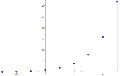
We have spent plenty of time so far reasoning about repeated multiplication, and how to generalize this idea. However, some good visual intuition would be nice: what does the exponentiation process look like? The easiest base to picture is 2, so we will look at the function 2^x. For each value of x, this guy spits out the value of 2 raised to that power. Using our rules above, its easy to calculate this for x an integer; you just start with 1 (which is 2⁰) and double it to get 2¹, then again to get 2², and so on. This gives the set of values

到这里我们已经花费了大量的时间去讲解重复性的乘法，以及如何拓展其适用范围。然而，如果能有一些可视化的直观理解就更好懂了。做指数运算的过程是什么样的？最容易理解的底数为2，所以我们看一下指数函数 2^x.x取任意值，这个函数就给出2的x次方的值。利用我们上面所讲的指数计算的规则，当x为整数时很好计算，我们从1开始，此时对应于2⁰，然后乘以2得到2¹,再乘以2得到2²,如此往下计算，得到一些列的值，如下表所示

，

x	-2	-1	0	1	2	3	4	5	6
2^x	1/4	1/2	1	2	4	8	16	32	64

Which can be plotted on a graph to better visualize the dependence

我们可以把这些值画成图

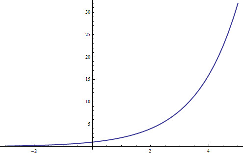
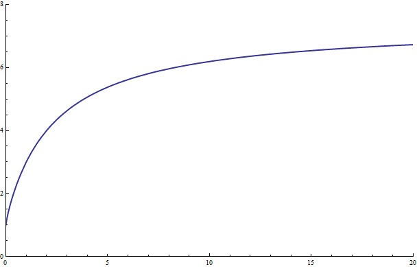
This graph can be further "filled in" by plotting all the remaining points, giving a graph of 2^x for all real x.

上面的离散的点之间可以通过填充得到一条线，从而我们可以得到函数2^x的函数图像，x为任意实数

Having already uncovered the algebraic intuition behind the laws of exponents, lets see if theres any way to understand them geometrically. Instead of motivating the rule

$a^m \cdot a^n = a^{m+n}$ by considering the special case of m and n being integers, we will try and look at this in terms of the graph of the function a^x. As an example, lets take a=2. What happens if we multiply each point on the graph by two? This would amount to a vertical stretching of the graph, moving each point twice as far from the x axis as it originally was. Algebraically, this new function is $2 \cdot 2^x$ , which by the laws of exponents can be rewritten $2^{x+1}$ . Quick recap: our original function was $2^{x}$ , and we doubled it to get $2^{x+1}$ . However this is simply the original function shifted to the left by 1. Thus stretching vertically by a factor of 2 produces the same result as shifting the graph to the left by 1. This is shown below.

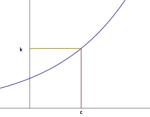
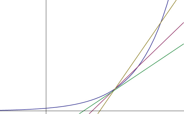
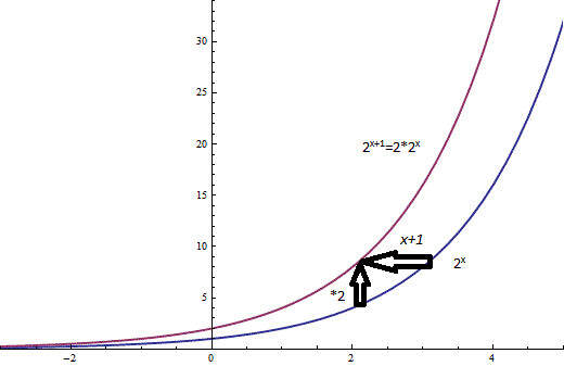从代数的角度理解了指数运算过程中的那些规则以后，让我们看看能不能从几何角度去理解它们。为了得到 $a^m \cdot a^n = a^{m+n}$ 这个指数运算的规则，我们并不需要从m和n为整数这种特殊的例子开始往下一步一步拓展。我们直接从图像的角度来看指数函数a^x.举个例子，比如a=2。如果我们把图像上的每个点都乘以2（确切地说是图像上的每个点的y值都乘以2）会怎么样？这就相当于一个垂直方向的拉伸，将图像中的每个点拉伸到原来距离x轴距离的2倍。代数上此时的新函数为 $2 \cdot 2^x$ ，根据指数运算的规则，可以简化成 $2^{x+1}$ 。简单提醒一下，我们初始的函数为 $2^{x}$ ，我们将它乘以2得到了函数 $2^{x+1}$ 。然而将原函数左移1个单位长度是更容易的一件事，左移1个单位长度也可以得到 $2^{x+1}$ 。所以对于函数 $2^{x}$ 垂直方向拉伸2相当于左移1个单位长度。对上面描述的演示如下图：

This is a special property of exponentials; their self-similarity. Stretching one vertically is equivalent to translating it horizontally instead. Lets see to what extent this is true. Lets pick some arbitrary exponential a^x, and some point P on its graph (this is the blue graph in the figure below). If we let r denote the x-coordinate of P, the y-coordinate of P is simply a^r. Now lets stretch this entire graph vertically by a factor k. The new graph, $k \cdot a^x$ is purple in the below figure. If k is a positive number, then we can find some number c such that $k=a^c$ . This allows us to re-express $k \cdot a^x$ as $a^c \cdot a^x$ , or equivalently $a^{x+c}$ . Thus we have the relation

这是指数函数的一个特殊的性质：自相似性。垂直方向的拉伸相当于水平方向的平移。让我们看看这个性质在什么情况下是有效的。让我们随意拿一个指数函数a^x,在函数图像上随意取一个P点（如下图蓝色图像上的P点所示）。如果r是P点x方向的坐标，那么P点坐标的y值为 a^r.现在让我们将这个函数图像垂直拉伸k倍，新的函数图像对应的函数为 $k \cdot a^x$ ，在下图中用紫色图线表示。如果k是正数，那么我们总可以找到某一个值c，使得c满足条件 $k=a^c$ 。那么我们可以将函数 $k \cdot a^x$ 写成 $a^c \cdot a^x$ ，或者化简一步，写成 $a^{x+c}$ 。那么我们有如下关系：

$k \cdot a^x = a^{x+c}$

If we let Q denote the point on $k \cdot a^x$ which is the stretched image of P, this gives us a second way of getting to Q from the original graph: we can start at the point r+c on the x axis, and move vertically to a point R on a^x. Shifting this point horizontally c units to the left gives the point Q, which is a translated image of R.

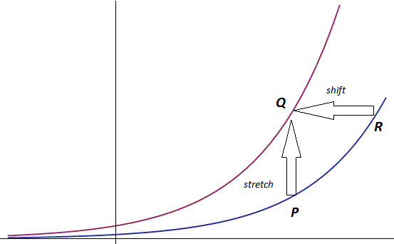如果我们用Q来表示函数 $k \cdot a^x$ 图像上的点，即为P拉伸过后得到的点，那么从P得到Q我们可以有第二种方式：我们从横坐标为r+c处找函数a^x上的点（假如这个点我们命名为点R），向左水平平移c个单位长度就得到了点Q，Q就是R平移以后对应的函数 $a^c \cdot a^x$ 上的点。

The geometric interpretation of the first "law" of exponents can then be stated as follows: if f(x) is some exponential function, then a stretch of the form kf(x) is equivalent to a translation of the form f(x+c). This is a property that can be observed on a graphing calculator or with a computer algebra system: as you zoom in on an exponential curve, provided you scale the axes right, it looks the same at any size. This self-similarity is the basis of the "memoryless" property of the exponential distribution often quoted in statistics, and will help us understand exponential derivatives in a bit.

第一条指数运算规则的几何上的解释可以表述为：如果f(x) 是某个指数函数，那么f(x) 在y方向的拉伸版本kf(x)等价于f(x)的平移版本 f(x+c)。这个性质可以在绘图计算或者计算机代数中观察到：当你放大一个指数函数的曲线的时候，假设你放大x轴，那么在任何放大倍率下图线看起来都是一样的。这种自相似性是统计学中经常提到的指数分布的“无记忆性”的基础。[“无记忆性”翻译的太直接了，但我不知道在统计学中怎么称呼，所以就先放在这里]。这也有助于我们理解指数函数的导函数。[一直认为“导函数”的翻译无法带来任何有助于理解这个东西是什么的任何一点点的帮助，导函数其实就是每个点处的斜率值作为函数值画出来的函数]

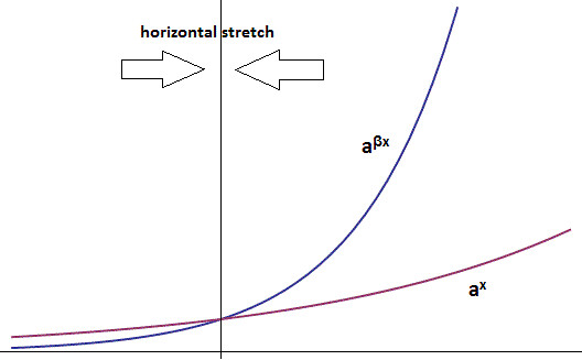
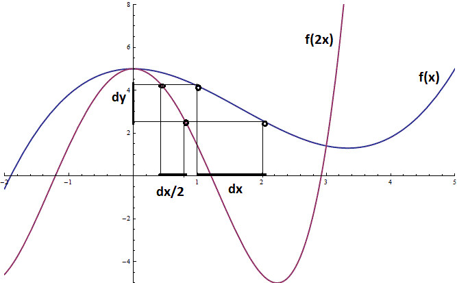
We have taken a look at what happens when we stretch an exponential vertically, but what about if we stretch it horizontally? A horizontal stretch is a stretch of the x-axis, and so we can accomplish it algebraically by replacing x with bx in our formula. For b<1, this corresponds to an expansion, and b>1 is a contraction, or squishing of the graph about the x-axis origin. This is illustrated below.

我们已经看了当我们竖直方向拉伸或者压缩指数函数时发生了什么，那如果我们横向对指数函数做伸缩呢？横向的伸缩就是x方向的伸缩，公式中我们可以用bx代替x来表示x轴方向上的伸缩。当b<1时，对应于x方向的拉伸；b>1时对应于x方向的压缩。示意图如下：

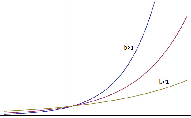From the above pictures, it appears reasonable to assume that a horizontal stretch (either compression or expansion) produces yet another exponential function. To take a concrete example, lets go back to our old friend . $2^x$ This graph can be horizontally compressed by replacing x with 2x. These two exponentials are shown below.

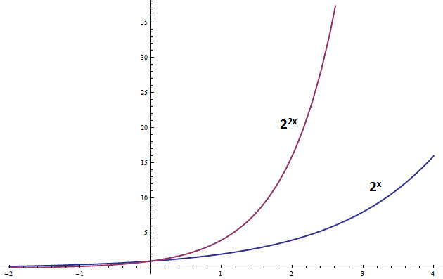从上面的图中我们可以看到，有理由假设横向伸缩以后得到新的指数函数的图像。举一个具体的例子，还是拿之前用过的例子 $2^x$ 为例吧。这个函数可以横向压缩，体现在公式上是把x替换成2x。压缩前和压缩后的图像如下图：

Because throughout our extension of exponentiatiton from the integers to all real numbers we forced the identity $(a^m)^n=a^{m n}$ to hold, we can use this to re-express our compressed exponential in a more insightful way. In terms of the example,

因为我们在将指数从整数拓展到全体实数的时候保证 $(a^m)^n=a^{m n}$ 这个运算操作公式依旧是适用的，所以我们可以换一种写法换一钟标记形式，从而可以更直观的揭露“压缩”这个操作的本质。

$2^{2x}=(2^2)^x=4^x$

And so a horizontal compression is equivalent to a change of the exponential base. When thought of in terms of functions, this is the geometric interpretation of the equation $(a^m)^n=a^{m n}$ . Given an exponential $a^x$ , the effect of a horizontal stretch $x \mapsto b\cdot x$ is really just a change of base. If we let c stand for the value of $a^b$ , then a stretch of factor b is equivalent to the change $a^x \mapsto c^x$ .

从上式可以看出，横向的伸缩变换等价于指数函数底数的变化。这也是从图形角度理解 $(a^m)^n=a^{m n}$ 。给定一个指数函数 $a^x$ ，横向的伸缩变换 $x \mapsto b\cdot x$ 只是底数的变换。如果我们令c代表 $a^b$ 的值，那么拉伸b倍（或者压缩为原来的1/b）等价于 $a^x \mapsto c^x$

Thus we have two ways to look at the rules for manipulating exponents: either we can view them algebraically as simply facts about what must be true for integer exponents to make intuitive sense, or we can view them as statements about how vertical and horizontal stretches of an exponential graph really end up resulting in translations or changes of basis. The ability to get from one exponential to another by two quite different means is a pretty useful property for intuition: in fact, these properties allow you to look at any exponential whatsoever as just a squished copy of some other exponential. To see this, we are going to need to know a little about undoing exponentials; so i'll pick up on this train of thought again in a bit.

现在我们有两种方式去看待运算指数函数时的操作规则：我们可以从代数的角度去理解，指数为整数如何运算，那么指数为实数就如何运算；或者从另一个角度，指数函数只是横向或者纵向的伸缩只是底数的变化或者整体图形的平移。有两种方法可以从一个指数函数变化为另一个指数函数。指数函数的这个性质可以给你提供一种思路：你可以把任意的指数函数看所某个指数函数的拉伸或者压缩。[这段后半部分先暂时不翻译]

Undoing exponentiation

反向的指数运算

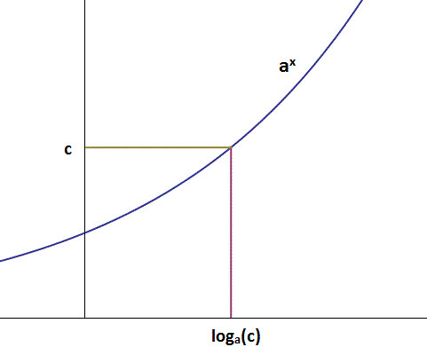
In the last section at one point, we had a number k, and we claimed that it was possible to rewrite this as $k=a^c$ for some c. Why can we do this? A quick picture will help here; plotted below is an arbritrary exponential curve, with some number k selected along the y axis. Looking at the corresponding x value (call it c) we notice that for this particular choice, $k=a^c$ as required. So long as k>0, this argument applies in general; its easy to see that there will always be some corresponding x value.

在上一个章节，我们设定了一个数字k, 并且设定对于任意的一个c总能找到对应的k，使得 $k=a^c$ 。为什么我们可以做这样的设定？用图片来演示一下。下方画的是任意一个指数函数的图像，和在y轴上任意选的一个k值，那么这个函数的y值为k时对应的x轴上的点（称之为c），在这种情况下， $k=a^c$ 。只要k大于0，总能找到在x轴上找到某个点c满足 $k=a^c$

Finding such a c for a given k is an inverse problem (given the output of the function, k, find an input c such that f(c)=k), and thus we are in need of an inverse function for the exponential. Since all exponentials are bijective functions, they are invertible, and we can actually do this. Geometrically an inverse function is simply the reflection of the original function over the line y=x; a graph of both an exponential and its inverse is shown below.

对于任意给定的k，找到对应的c值，这是一个指数函数的反向运算（就好像一个函数，给定他的输出k，反过来求他的输入c，使得f(c)=k）。所以现在我们需要指数函数的逆运算。因为所有的指数函数为bijective function[不知道怎么翻译这个词]，所以他们是可逆的，并且我们也确实能找到逆函数。从图形上看，一个函数的逆函数的图像是其关于 y=x的镜像。下图画出了指数函数和他的逆函数的函数图像。

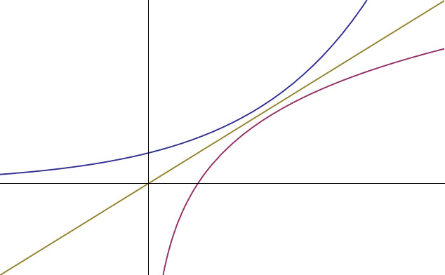To not wander too far astray, we won't spend too much time worrying about the inverse function, hopefully the above illustration is enough to provide some feeling that it exists (the proof is simple; just verify the injectivity and surjectivity of the exponential as a map $\mathbb{R}\rightarrow \mathbb{R}^+$ ). Now that we know there is one, to be able to discuss it precisely we need a good notation for it. If we have the exponential $a^x$ , then we will denote its inverse by $log_{a}(x)$ , and call such a function the logarithm with base a. This function is defined exactly like the first picture in this section; if b and c are numbers such that $a^b =c$ , then $b=log_{a}(c)$ . Pictorally;

为了不岔开话题太远，我们不会在逆函数上花费很多时间，希望上面的演示足够提供一个他的逆函数肯定存在的直观上的感觉（证明过程是简单的，只需要just verify the injectivity and surjectivity of the exponential as a map $\mathbb{R}\rightarrow \mathbb{R}^+$ ）。现在我们知道肯定有一个逆函数，为了讨论起来方便，我们需要用一个标记来指代他。如果我们有指数函数 $a^x$ ，那么我们把他的逆函数用 $log_{a}(x)$ 来指代，并把他的逆函数称之为以a为底数的对数函数。这个函数的定义与本小节第一张图片展示的完全一样。设定b和c是数字，并且满足 $a^b =c$ ，那么 $b=log_{a}(c)$ ，从图像上看如下所示：

Rewriting exponentials

重写指数函数

Ok, we've covered enough stuff now to discuss how the self-similarity properties of exponentials allow us great freedom in how we write them (and interpret them). Lets say for some reason or another, you've found a particular exponential function that you really like, call it $a^x$ . You're working on some problem and another exponential shows up; something that superficially bears no resemblance to your favorite member, we'll write this guy $b^{(x+c)}$ . There might be good physical reason that this exponential has the form it does, but no matter; whatever the source of this particular exponential there is a way to interpret it as simply a stretched copy of your $a^x$ . To see this, lets first consider the form of the exponential you were given. It is the simple exponential $b^x$ , after a horizontal shift of c units to the left. We know from previously that a horizontal shift is really just a vertical stretch, and so we can think of $b^{(x+c)}$ as being $r\cdot b^x$ , for a vertical stretch factor r (this stretch factor can easily be seen to equal $b^c$ ).

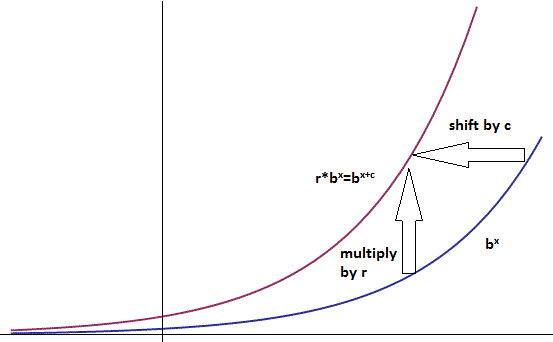好，我们已经回顾了足够多的资料，现在我们去讨论指数函数的自相似性是如何给了我们在表达形式上的极大自由度的。假如因为某个原因，你发现一个很喜欢的指数函数，比如我们叫它 $a^x$ ，你在解决一个难题，在解决这个难题的过程中遇到了另一个指数函数，这个指数函数跟你喜欢的那个一点也不像，我们用 $b^{(x+c)}$ 来表示新遇到的这个指数函数。也许新遇到的这个指数函数这种表示形式对应于实际的物理意义，但是没关系，无论这个指数函数怎么来的，都可以简单解释为你最爱的函数 $a^x$ 的伸缩版本。为了证实确实可以做到这些，我们先看一下我们拿到的指数函数的形式： $b^{(x+c)}$ 。这是指数函数 $b^x$ 经过水平移动c个单位长度后得到的。我们之前已经知道水平移动其实就是垂直方向的拉伸，那么我们可以把 $b^{(x+c)}$ 认为 $r\cdot b^x$ ，其中r表示垂直方向拉伸的幅度（这个垂直方向拉伸的幅度显然等于 $b^c$ ）

Now what about the remaining exponential? It is still the wrong base; so we need a way of viewing $b^x$ as some stretched copy of $a^x$ . We saw previously that change of base is really just a horizontal stretching, so we know that theres a way to write $b^x$ in the form $a^{\beta \cdot x}$ , for some horizontal stretch of magnitude $\beta$ . The value of $\beta$ satisfying this can be found using the exponent laws: we want to satisfy the equation $b^x=a^{\beta \cdot x}$ , so we need $b=a^\beta$ . If we now view $\beta$ as a variable in the exponential function with base a, we have a situation that has already been discussed: we know the y-coordinate of some point on the exponential curve $a^x$ , and we want to find the x coordinate. This can be accomplished using the inverse function; giving us our answer $\beta = log_{a}(b)$ .

那现在剩下的指数函数的部分该如何处置呢？底数还是跟我喜欢的那个不一样呀。我们需要把 $b^x$ 看做 $a^x$ 的伸缩版。之前我们看到底数的变换其实就是横向的伸缩。所以我们能找到把 $b^x$ 写成 $a^{\beta \cdot x}$ 这种形式的方法。其中 $\beta$ 是横向的伸缩幅度。 $\beta$ 的值可以用指数函数的定律来找到：我们想找到 $\beta$ 使得 $b^x=a^{\beta \cdot x}$ ，那么我们需要 $b=a^\beta$ 。如果我们把 $\beta$ 能做以a为底数的指数函数的变量，那么此时的这种情况我们已经讨论过：我们知道指数函数 $a^x$ 的输出值y，我们想找到对应的x使得输出值为y。这可以用逆函数来求解，从而得到 $\beta = log_{a}(b)$

Thus we have the formula

所以我们得到了公式：

$b^{(x+c)}=r\cdot a^{\beta \cdot x}$

and the values of r and $\beta$ which satisfy it, allowing us to view our arbitrary exponential as really just our old friend $a^x$ , stretched horizontally by $\beta$ and vertically by r. Below is an animation of how the two stretches in unison actually achieve this:

和满足这个等式的r和 $\beta$ 的值。这使得我们可以将任何一个指数函数看做我们的老朋友 $a^x$ 经过横向伸缩 $\beta$ ，然后纵向伸缩r得到的指数函数。下方是一个动画，用来演示如何通过两个方向的伸缩变换实现将任意指数函数转化为我们熟悉的指数函数的.

Exponentials and growth

指数和增长

Our first introduction to exponentials was their discrete nature, as an extension of multiplication. However this is not the only situation in which they arise, heck it's not even what makes them most useful. Passing from an algebraic shorthand to their continuous case left us with a set of functions over $\mathbb{R}$ with some pretty cool properties. One of the most useful interpretations of exponentials is that of growth, they are the natural choice of a mathematical model for a kind of growth which depends on how much "stuff" is already present. To see this, we will first take a step back and consider the nature of growing things in general.

我们第一次介绍指数函数是从同一个数的多次乘法来入手的，但是这并不是指数函数被提出来的唯一场景，也不是指数函数可以发挥最大作用的场景。从代数方面的简写形式到拓展指数的范围为连续的数值，指数函数有很多有意思的性质。其中一个很有用的解释是增长率。有一种增长模型是增长率由现有的数量决定，描述这种增长模型自然而然会选择指数函数这种数学模型。为了证明确实如此，我们首先回顾一下一般意义上的增长的本质

The simplest kind of growth is linear growth: say each day you are given a dollar from your friend. After 5 days, you will have 5 dollars, after x days, you will have x dollars. Your riches grow linearly with time. The amount of money you will make tomorrow doesn't depend on how much money you have today; regardless of if you are broke or a millionaire, you will make one dollar tomorrow. Now lets consider a different scenario: someone gives you a dollar, and you invest it in some ridiculous company which promises to double your total investment each day. So, the next day they give you a dollar, doubling your current amount. The second day however, they give you 2 dollars, so you now have a total of 4. The following day they double that, giving you 4 so that you have 8. Continuing this process, you see that your dollar amounts each day form the list {1,2,4,8,16,32,64,....}, which is nothing other than the table of values for 2^x. In this model of growth, the amount you earn tomorrow depends on how much you have today: if you have 1 dollar you will make a dollar, if you got a million, you'll make a million. The striking difference between these two modes of growth can be seen below

。最简单的增长是线性增长。假如每天你的朋友给你一块钱。五天以后你就有五块钱，x天后你就有x块钱。你的财富增长与时间是线性关系。明天你将得到多少钱与今天你有多少钱无关，假如你没有破产也不是亿万富翁，你明天会挣1块钱，现在让我们考虑一下另一个场景：某人给你1块钱，然后你把这1块钱投资给了一家公司，这家公司承诺说每天会将你的投资总额翻倍。第二天，因为你投入了1块钱，他们将给你1块钱，你的账户里将是2块钱。第三天，因为你的账户里是2块钱，所以他们给你2块钱，你的账户里是4块钱。再下一天，他们会给你4块钱，现在你的账户里有8块钱。持续这个过程，你会发现账户里的钱每天变化，1,2,4,8,16,32,64……,这些点其实就是指数函数 2^x

上的点。在这种增长模型下，你明天挣的钱将取决于你今天有的钱。如果你有1块钱，你将挣1块钱，如果你有一百万，你将挣一百万。这两个增长模型的差异如下：

Looking at exponentials as a form of growth allows a nice physical interpretation of the "vertical stretch = horizontal shift" we talked about: say you're that lucky investor whose total investment is doubled each day. If you start on day 0 with 1 dollar, your income is modeled by 2^x. But what if you started by investing 8 dollars? your income on day 2 would be 16 dollars, making your total 32, your total the next day would be 64, then 128, and so on. In fact, each day you will be making as much money as the guy who invested a single dollar does 3 days later. Your income is simply his income shifted by 3 days. Thus investing 8 dollars to begin with (stretching the income function by a factor of 8 vertically) is the same thing as just having invested a single dollar 3 days earlier (shifting the income function horizontally by a factor of 3).

把指数函数当做描述增长过程的模型给了我们对指数函数的性质“垂直方向的拉伸=水平方向的移动”一个直观实际的解释：假如你是一个幸运的投资者，你的投资每天都会翻倍。如果你在第0天投资1块钱，你的收入可以用 2^x

这个函数来描述。如果你最开始投入的是8块钱呢？你第二天的收入将为16块钱，此时你的总账户余额为32块钱。下一天你的账户余额将为64块钱，然后是128块钱，如此等等。事实上，你每天的收益是原来每天投资1块钱时对应3天后的收益。相当于把投资一块钱时候每天的收益平移了一下。所以开始投资8块钱（与开始投入1块钱相比是将收入函数垂直方向拉伸8倍）等价于提前三天开始投资投资初始额度为1块钱（将每天的收入函数水平平移3）

In fact, any growth process where your amount of growth is proportional to how much you have at the moment is a form of exponential growth. Tripling your total amount each day is the exponential 3^x, quadrupling amounts to 4^x. Heck even multiplying your total by 12.3456 (or any other random number) each day is modeled by the function (12.3456)^x.

事实上，任何增长过程，只要他的增长速率与当前所拥有的数量有一个比例关系，那么就可以用指数函数来描述。每天收入翻三倍，可以用指数函数3^x来描述。每天翻四倍，可以用指数函数4^x来描述。每天的收入是现有的余额乘以 12.3456，可以用(12.3456)^x来描述。

These examples have all been of the discrete case, but the same intuition carries over to the continuous case: if you have a growth rate which is proportional to the amount of stuff you have, the growth will be exponential. We can formulate this more precisely in the language of differential calculus: let y(t) be a function which for each time outputs an "amount". At a given time t*, the rate at which y is growing is its derivative, y'(t*). To say that the growth rate is proportional to the amount of stuff you have, is to say that the derivative is proportional to the function's value at that point

这些例子中变量都是离散，一个一个单独的数字，但是这些例子中的规律也适用于变量为连续的情况、假设增长率与现有的数量成正比，那么这个增长将为指数型增长。我们可以用微积分更精确的描述：令y(t) 是一个函数，每次输出一个值。在某个时刻 t*下，y增长的速率就是他的导数 y'(t*)。当我们说增长率与现有量成正比的时候，我们其实是在说函数的导数与现有量成正比。用公式写下来如下：

$y'(t)=r\cdot y(t)$

t时刻的增长率=一个数字*t时刻的拥有量

The functions y(t) which satisfy this are the exponentials that we have been discussing all along (I wont bother deriving why....the usual proof involves knowing that a certain integral comes out to be the natural logarithm; a fact that here doesn't help much with intuition). Hopefully the analogy of this differential equation with the discrete case is at least suggestive that both should follow the same general trend.

满足这个公式的函数y(t)是指数函数，我们已经讨论过指数函数了。（括号中的先不做翻译，后面的先不做翻译）

That special number "e"

特殊的数字e

It seems you can almost not hear of or work with exponentials without encountering that seemingly random irrational number, 2.71828182....=e. It's one of those things that is mystifying the first few times you see it, but it comes up so often that before long it is second nature to use. However, during the learning process (at least in my experience) using e for years never really gave a good sense of exactly what made it special. e is singled out for multiple different reasons, which is probably why it's hard to see any underlying theme when learning to use it. Throughout the rest of this article I'm not going to try and present proofs or derivations of e in full detail, but rather discuss some of the situations where it arises naturally in a more casual manner.

涉及到指数函数的工作，几乎没有不用到一个特殊的数字e 的，e=2.71828182....前几次遇到数字e的时候总是会感到迷惑，见得次数多了你会发现经常用到它。然而，几年来我对e的学习和使用并没有让我对它有一个很好很精确的理解。e之所以如此特殊是因为很多原因，这也是为什么在学习使用他的时候很难看到隐藏的本质。在接下来的文章里我并不打算给出证明并对e做一些具体的拓展性讲解，而是讨论一些场景，在这些场景中数字e自然而然的被提出来。

First of all, you may ask, why would there even be any "special" base for the exponential? What has been discussed so far has been done in full generality; with a serving as a placeholder for any base you could want. In this sense, it seems that all possible exponentials are created equal. Sure, we can pick some a that we like and write all exponentials as just stretched versions of it; and this might be a very convenient thing to do (computationally you would only ever have to worry about one exponential function, and just feed it different arguments), but how could there be a natural way to select such a base? My goal here is to convince you that there is a natural choice, that the choice is e, and that the various ways of defining this number actually share a common theme.

首先，我们也许会问，指数函数中为什么会需要特殊的底数？迄今为止的探讨已经足够具有一般性，底数可以是任意的值都满足我们刚才讨论的指数函数的行为性质。从这个角度来看，似乎所有的指数函数都是平等的。当然，我们可以挑选我们喜欢的底数构建指数函数，并将其他所有的指数函数写成这个指数函数的伸缩版本。这看起来非常的方便（计算的时候你只需要关注1个指数函数就可以，变化的只是这个指数函数里面的一些参数），但是，有没有一个自然[或者翻译成“更接近本质”？]的方法去挑选指数函数的底数呢？我希望能说服你确实有一个自然而然的选择底数的方法，并且这种方法选出来的底数为e，各种各样定义这个数字e的方式本质上描述的都是相同的东西。

Lets start back with the idea of exponentials representing growth: out of all discrete growth rates, the one singled out as "special" is the unit growth rate; or an increase of 100% of your amount each day. This is our friend 2^xfrom before, but lets see why. As we argued before, discrete exponential growth is a process where the gain over each unit of time is proportional to the current amount:

让我们回顾一下用指数函数来表示生长速度：在所有生长速率中，有一个生长速率比较特殊，即为单位生长速率，或者说是每天增长100%。这是我们之前比较熟悉的 2^x，我们来看看为什么他如此特殊。正如我们之前讨论的，离散的指数增长是单位时间内的增长量与当前拥有量成比例关系。简洁的表达如下式

$gain \propto value \Rightarrow exponential$

增长量正比于当前拥有量——>描述这种增长方式的函数为指数函数

Say the current value on a given day is P. Since the gain on the next timestep is proportional to P, we can write gain=rP for some proportionality constant r. The amount you have at the end of that next time step is then the previous amount plus the gain: P+rP. We can factor the current amount out of this equation, giving (1+r)P. This gives the total amount at a given time in terms of the amount at the previous time. Letting P vary with n;

假设某天当前的拥有量为P。因为下一个时间间隔内（或者说时间块）的增长量与当前拥有量P成正比，我们可以写成增长量=rP ，r是任意一个小数，用来表示增长量与当前拥有量的比例关系。在下一个时间间隔截止的时候（或者说在下一个时间块的末尾处），当前的量为之前的拥有量P加上增加量rP ，即为P+rP ，提取公因式P，写成(1+r)P 。这就给出了在某个时刻下的拥有量和前一个时刻的拥有量。假定P只与n有关，即P为n的函数，n是第几个time step，或者说n是第n时间块。

$P(n+1)=(1+r)P(n)$

第n+1个时间块以后当前的拥有量=（1+r）乘以第n个时间块后当前的拥有量

Solving this recurrence relation gives

解这个递归方程得到下式：

$P(n)=P(0)\cdot (1+r)^n$

第n个时间块时当前的拥有量=最开始时的拥有量乘以 (1+r)ⁿ

Which gives the amount at all future times in terms of the initial amount in terms of a stretched exponential with base 1+rate. Setting the rate of growth to unity (that is, making the proportionality above an equality), gives us the equation $P(n)=P(0)\cdot (1+1)^n=A\cdot 2^n$ , which justifies the fact that discrete growth at a unit rate is modeled by 2^x.

上式给出了未来任意一个时间的拥有量，这个拥有量与最开始时的拥有量和底数为(1+增长率)的指数函数来表示。令增长率为1，得到式子 $P(n)=P(0)\cdot (1+1)^n=A\cdot 2^n$ ，印证了离散的增长速率下单位增长速率的情况可以用2^x作为增长模型来描述

The natural question is then, can we extend this notion of "unit growth" in some way to the continuous case? That is, is there any continuous exponential which we can say grows at unit rate? From our look at the discrete case we have learned two properties of unit growth which can be used to characterize it: namely that the proportionality constant between growth and current value is 1, or that at any instant in time the rate of growth is equal to the current value. How would we phrase these requirements in the continuous case? We saw before that if the growth rate is proportional to the value, we have the condition $y'(t)=r\cdot y(t)$ . Setting r to unity in this equation gives us a differential equation for unit continuous growth:

自然而然的，我们就有一个问题，能否把这种离散的每单位时间增长率为1的记号形式扩展到连续的情况？也就是有没有连续的指数函数用来表示以单位增长率来增长的情况？我们处理离散的情况观察到单位增长率的指数函数的两个性质：1、增长率和当前的拥有量的比值是一个常数，比如1，也就是说在任意时刻下增长速率等于当前拥有量。我们如何在连续的情况下表达满足这个性质的函数呢？之前我们看到如果增长速率与当前拥有量成正比，那么我们就可以得到表达数量关系的式子 $y'(t)=r\cdot y(t)$ 。另r为1，那么我们就得到了增长率为1时的微分方程

$y'(t)=y(t)$

t时刻的增长率=t时刻的拥有量

The solution to this equation will then be the function which we can say grows with unit speed. Since we know by the equation's form that it is an exponential; all we must do is find which base satisfies it. For lack of a numerical value, lets call the base e. Stepping back from our current question about growth rates and looking at the equation itself, it turns out we have run into another quite interesting problem. This equation selects functions y which are their own derivative. That is, unit growth is equivalent to the condition that the differential operator have no effect on the function. Without considering our reasoning that got us to this equation, it may seem unlikley that it has a solution at all: after all, if it does that means that there must be a function out there which remains invariant under differentiation. However phrased in terms of growth rates, we know there are exponentials with growth rate less than 1, and those of growth rate greater than 1; so it makes intuitive sense that there should be some exponential in between, with growth rate of exactly 1. Thus for now, we are going to assume this equation is solvable, and see what we can learn about the qualities of its solutions.

这个微分方程的解就是我们所说的按照100%的增长率增长的函数。根据这个微分方程的格式加上之前所讲的，我们知道这个微分方程的解是指数函数，现在我们需要做的只是找到一个合适的底数来表示这个指数函数。我们暂时把我们要找的这个底数称之为e。回顾一下我们当前关于增长率的问题和这个公式本身，发现我们转化成了另一个问题。这个公式把函数值y作为他的增长率。换句话说，单位增长率意味着求导数（其实就是斜率）的操作并不会对函数造成影响。看起来这个方程应该是找不到解的，因为如果这个方程存在的话，就会有一个函数在做求导时是保持不变的。但是如果考虑到增长率，我们知道有的指数函数是增长率小于1的，也有增长率大于1的，所以应该就有增长率等于1的。那么现在我们假设这个方程是可以求解的，那么他的解有什么性质呢？

Looking at the differential equation, we see that it is first order in t. Without initial conditions, this implies that there is a 1-parameter family of solutions to this equation, which we will index by a and let $Y=\{y_a(t)|a\in \mathbb{R}\}$ . Also, this equation only mentions the derivative at t and the y-coordinate at t, never the actual t value at which they occur. Because of this, we can see that given a particular solution of this equation, say y(t), then y(t-a) is also a solution (use the chain rule).

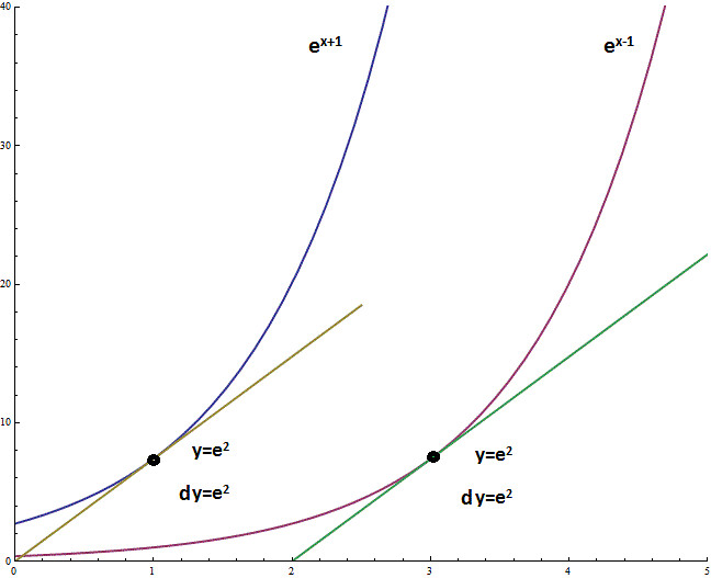观察这个微分方程，可以知道是关于t的一阶。没有初始条件限制，那么会有一些列的解，这一系列的解之间差一个常数，假如我们称这个常数为a，那么微分方程的解可以表示为 $Y=\{y_a(t)|a\in \mathbb{R}\}$ ，这个式子只是提到了微分方程的解在t时刻的导数和t时刻的y坐标，并不是确切的某个时刻t。那么我们知道给他任意的一个解，比如说y(t), 那么y(t-a) 也是一个解。

This tells us that the solutions to this equation are all related to eachother by the translation of one basic solution to the left or right. Since we additionally know the solution must be exponential, we can use our geometric interpretation of the laws of exponents to notice that shifts to the left or right are equivalent to vertical stretches. This lets us write our one parameter family of solutions as

所以我们知道所有这个方程的解都是其中一个解左右平移得到的。因为我们也知道这个解一定为指数函数，我们可以用之前提到过的从几何角度对于图形变换的解释——左右平移等价于垂直方向的伸缩——来将我们解表达出来，即为将所有的平移转化为y方向的伸缩。

$y_a(t)=a\cdot e^t$

与变量t和常数a有关的函数y=a乘以e的t次方

How do we go about finding the value of this e? Lets look quickly back to the discrete case for some help. Considering our unit discrete growth function of $2^n$ , look at the discrete analog of the derivative at a point, the slope of the secant line defined there. At a given n, we have

我们如何找到e的具体值呢？我们回头看一下离散的增长情况。考虑一下我们离散的单位增长率的函数 $2^n$ 。看一下求离散的函数 $2^n$ 其中一点的切线的近似类比，当然这里只能称之为割线。对于一个给定的n，我么可以得到：

$\Delta(2^n)/\Delta(n)=\frac{(2^{n+1}-2^n)}{(n+1)-n}= 2^{n+1}-2^n=2^n$

函数 $2^n$ 的值的变化量/n的变化量= $2^n$

Thus, the secant line at a point is equal to the value of the point (sounds rather like the differential equation we have constructed for the continuous case!). Lets see if we can't phrase this somehow in the continuous case. Instead of starting with the full blown differential equation, lets consider the slope of the secant lines of a graph as they approach the derivative. To match the discrete case (and follow our differential equation) we want

也就是说函数 $2^n$ 上任意一个点的割线的斜率等于这个点的函数值（听起来像我们刚才给连续类型的函数构筑的微分方程）。让我们看看能否用同样的术语描述连续的case。不用成熟的微分方程，我们考虑一下当割线的另一点接近于我们关注点的割线。为了与离散类型的例子相一致，我们用如下式子表示

$\lim_{h \to 0}\frac{e^{x+h}-e^x}{h}=e^x$

h无限趋近于0即为当割线的另一个点无限趋近于0的时候，割线的斜率=所求割线的点处指数函数的函数值。这个指数函数的底数用e来表示

也可以理解成对于任意的一个点x处的斜率（也就是增长率）=该点处的函数值

Considering at first finite values of h, we have a sequence of secant lines whose slopes approach the derivative of our graph at x.

假设现在有一系列越来越小的h值，那么每一个h值都可以对应一个割线，随着h值的减小，割线的斜率越来越接近x处的切线的斜率。

Lets see if we can use this equation for the slope of a secant line to solve for the correct base e. Muliplying through by h and dividing by $e^x$ ;

我们看看能否用这个求解割线斜率的公式来求的底数e的准确值。左右乘以h然后除以 $e^x$ ，得到下面的式子：

${e^{h}-1}= h$

This equation can be solved for e, yielding

这个等式可以用来解出e的具体数值，变换一下然后开方，注意前提是h无限趋近于0，所以用极限的表达式如下

$e=\lim_{h\to 0}(1+h)^{\frac{1}{h}}$

By considering the limit of secant lines of a graph under the restriction that the derivative must equal the value at that point, we have found an expression which will give us the value of our elusive "special" base. Calculating this limit numerically we arrive at

当h无限趋近于0时，割线率变化的极限值是此点处切线的斜率，通过这个数量关系，我们推导出来求解e的具体值的式子。通过求解这个式子（比如多试几个越来越接近于0的h）得到e的值为

$e\approx 2.718281828...$

以上是从斜率的角度来推导出来e代表的具体数值

To try and get some feel for another reason e is special, lets look at what happens when you have 100% growth divided over a unit time. The simplest case (that of no divisions at all) is just the discrete case from before: starting with 1 at t=0 after one time step we have a value of 2.

从另一个角度来感受一下为什么e很特殊，让我们来看下当你把100%的增长率平均分配到一个单位时间内会如何。最简单的情况，也就是把单位时间看作一步的情况，就跟之前一样。t=0时刻开始值为1，一个时间单位后因为增长率为100%所以此时的值为2

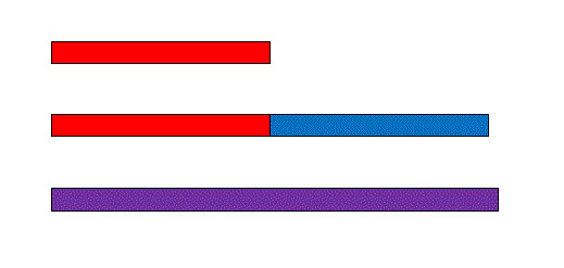What happens if we break the time step of the discrete case in half, first increasing by 50%, and then taking the output of this process and increasing it an additional 50%? This still gives 100% growth, but broken up into pieces. After this process; we have a final amount of

如果我们把时间段分为两部分更小的时间段呢？比如分为原时间段的一半，然后把第一个0.5时间段后的拥有值作为下面0.5时间段的初始值，增长率还是50%。最终增长率还是100%，但是分成了多份。经过这种类型的增长，我们得到的值为

$(1+\frac{1}{2})(1+\frac{1}{2})(1)=(\frac{3}{2})^2=\frac{9}{4}$

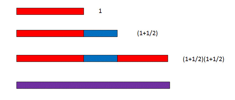Which is greater than the unbroken doubling which results in 2. What about breaking the time step into three pieces, and growing at a rate of 1/3 over each period? The result of this process is below:

这比1个时间段内增长率为100%得到的最终结果要多一些。如果把时间段均分为3份呢？每份时间内的增长率为1/3，这样增长的结果如下：

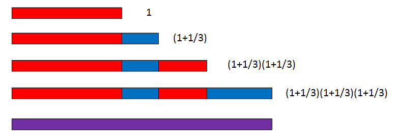$(1+\frac{1}{3})(1+\frac{1}{3})(1+\frac{1}{3})\approx 2.37...$

This is even larger than the previous division, which begs a question: does dividing 100% growth over the unit time interval diverge as the number of divisions tends towards infinity? If we divide the unit time interval into n pieces, and grow at a rate of 1/n during each step; we reach a final value of

这比将一个单位时间分成两份每份的增长率为0.5的情况下得到的结果要更多一些。那么问题来了：如果将单位时间无限细分，将增长率平均分配到这无限细分的时间内，会发生什么呢？如果我们把单位时间平均分n份，每份的增长率为1/n，那么我们得到了如下的式子

$\underbrace{(1+\frac{1}{n})\cdot ...\cdot (1+\frac{1}{n})}_\textrm{n}$

For n=100, here are the bars analogous to those above

n=100时，下面是用图形来表示上面式子的示意图

It appears at first that this may be diverging towards infinity. But, changing the value of n does not add more terms to the end of this sequence, but rather refines the sequence, making each individual bar smaller. The limit of these bars to zero width is then the model of continuous 100% growth that we are seeking. Looking over a wide range of n values, it appears that the value after unit time is tending towards a fixed number. Assuming this indeed happens, then breaking 100% growth into pieces and distributing it over smaller and smaller intervals results in a value of after one unit time step.

根据上面的图看起来似乎是随着将单位时间划分的越细，最后的结果会越来越大。但是增大n的值并没有将这一些列数字增大，而只是更精细了而已，也就是说每一个小横条更窄了。当这些小横条无限趋近于0时，这就是我们找的100%增长率且变量连续变化的模型。尝试很多次n的值，发现最终的计算结果趋近于一个固定的值。也就是说把100%增长率平均分成无限小的部分然后分配到将一个时间单位分成同样份数的时间间隔中，得到了一个固定的值

$\lim_{n\rightarrow \infty}(1+\frac{1}{n})^n$

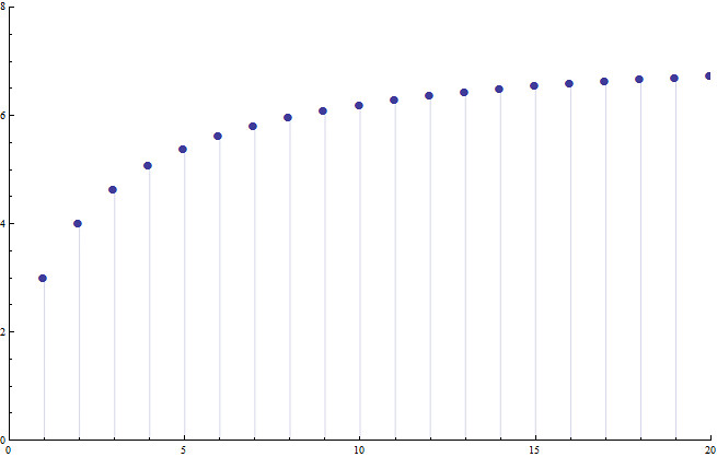
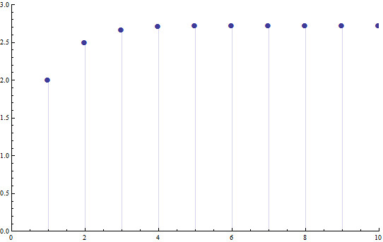
Numerically calculating this limit, we find

计算这个值我们发现：

$\lim_{n\to\infty}(1+\frac{1}{n})^n=2.718281828....=e$

Below is a plot of this limit:

下方是当n从1到很大时求解这个极限过程的示意图

横坐标为n，纵坐标是计算出来的值

This gives us the useful view of e as the limit of 100% growth over an interval, as the time steps become continuous. More importantly, as can be seen in the above graph, the sequence of points converging to e in the limiting expression are monotonic increasing: that is, e represents the maximum possible growth that can be obtained by dividing 100% over the unit interval. Not only is $e^x$ the expression for continuous unit growth, but also it is the maximal unit growth function out of all discrete and continuous versions!

这使得我们可以把e看做连续增长的情况下一段时间内100%增长率能增长到的极限。更重要的是从上面图中可以看到，可以看做这一系列的单调递增的点最后无限接近于e，也就是说e是单位时间内100%增长率能增长得到的最大值。 $e^x$ 不仅仅表达连续单位增长率，也是离散和连续增长情况下的最大情况。[这句好难翻译，翻译的不好]

The utility of e as a base

e作为底数的实用性

We have come across a few different mathematical reasons that select e as a rather special base for the exponential function; but it's most useful property is yet to come. If e represents the result of continuous 100% growth, what is the result of 50% continuous growth over an interval? Looking back at the above limit for e, we can see that breaking the original 100% up over n time steps resulted in the formula

选择e作为指数函数的底数，我们已经看了几种数学方面的原因。但是最实用的原因还没讲。如果e代表单位时间内连续100%增长率，那么单位时间内连续50%增长率得到的数字是什么？回顾一下上面用极限的思路求解e的过程，我们可以发现把100%增长率平均分配到n份时间内（将单位时间平均分成n份时间间隔）得到如下计算式子

$(1+\frac{1}{n})^n$

Likewise, distributing 50% growth over n time steps would produce a final result of

类似的，把50%增长率平均分配到n份时间（将单位时间平均分成n份时间间隔）应该得到下面的式子：

$(1+\frac{0.5}{n})^n$

Lets take a quick look at what this converges to as $n\to \infty$ :

让我们快速的看一下当n从1趋向于无穷时这个式子的值趋近于什么：

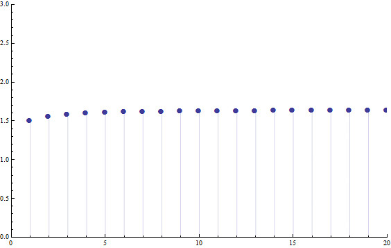In the limit, this comes out to approximately 1.6482. Is it a coincidence that this is precisely the square root of e? Definitely not! Let's see why:

To get to the limiting value of this expression; we don't need to consider all the terms; the limit just asks what happens "at infinity", so as long as we consider at least some of the terms way out there; we can see what happens (this can be made more precise by noting that since the original sequence is convergent, so are its subsequences). Before jumping into the whole subsequence stuff, lets just look at a relatively "big" term, by setting n=50.

这一系列数字的极限是1.6482。这恰好是e的平方根，是巧合吗？当然不是！让我们看看为什么：为了得到这个式子的极限，我们不需要求出所有的值，求极限仅仅关心无穷多个发生了什么，所以只要我们考虑几项，我们就能知道发生了什么（或者更确切的说因为原始的数列是收敛的，所以他的子数列也是收敛的）。在看所有的数字之前，我们先看看一个相对比较大的，比如n=50

$\left( 1+\frac{0.5}{50}\right)^{50}$

We can re-write this as follows:

我们可以变换这个式子写作

$\left( 1+\frac{0.5}{50}\right)^{50}=\left(1+\frac{1/2}{50} \right )^{50}=\left(1+\frac{1}{100} \right )^{50}=\left(1+\frac{1}{100} \right )^{100/2}$

The last term in this sequence looks a lot like one of the terms from our original sequence for e, except the exponent is divided by two. To make sure what we are witnessing here is something real and not just a coincidence; lets consider a much larger term: n=5000.

式子末尾变换得到的形式看起来就像我们求解e时候的其中一个式子，但是指数除以了2.为了确认一下情况，我们考虑一个更大的数字，比如另n=5000

$\left( 1+\frac{0.5}{5000}\right)^{5000}=\left(1+\frac{1/2}{5000} \right )^{5000}=\left(1+\frac{1}{10,000} \right )^{5000}=\left(1+\frac{1}{10,000} \right )^{10,000/2}$

This time we end up with the 10,000th term in the sequence for e (except we also have that factor of 1/2 in the exponent). Using what we know about fractional exponents however, raising something to the half power is the same as taking the square root. So these are just the square root of two terms in the sequence for e. If this pattern continues; then we can show that the base for continuous 50% growth is really just the root of e, as was suggested numerically.

这次我们变换之后得到的式子是逼近e的数列的第10000个数，当然指数还是除以了2.指数除以2意味着什么，意味着开方。也就是说刚才n=50和现在n=5000,计算出来的值是求解e的数列中对应数字的开方值。每一个值都是e对应位置数字的开方值，那么最终极限值也是e的开方值。

To make this exploration precise; lets take a specific subsequence of our limiting sequence, consisting only of the terms for which n=5x10^m. Since as m tends to infinity in this sequence n most certainly does as well, we will get the same limiting behavior. Lets look at the form of our new sequence:

为了更精确的表达这个思考的过程，让我们选择当n=5x10^m时的一列数字。因为当m趋近于无穷大时n也趋近于无穷大，我们会得到同样的极限。让我们看一下这一列数字的格式：

$\left( 1+\frac{0.5}{5\cdot 10^m}\right)^{5\cdot 10^m}=\left(1+\frac{1/2}{5\cdot 10^m} \right )^{5\cdot 10^m}=\left(1+\frac{1}{10^{m+1}} \right )^{5\cdot 10^m}=\left(1+\frac{1}{10^{m+1}} \right )^{10^{m+1}/2}$

Using our rules of exponents, we can re-write this last expression as

通过指数函数的规律做变换，我们可以把上面最后一步得到的式子变换为

$\sqrt{\left(1+\frac{1}{10^{m+1}} \right )^{10^{m+1}}}$

Now we have a new way to calculate our limit:

现在我们有了一个新的方法来计算极限：

$\lim_{n\to\infty}\left(1+\frac{0.5}{n} \right)^n=\lim_{m\to\infty}\sqrt{\left(1+\frac{1}{10^{m+1}} \right )^{10^{m+1}}}$

Because the square root is a continuous function, we can drag our limit right inside of it. The terms inside the root limit right to e however (they are just a subsequence of the sequence $(1+1/n)^n$ , and so they have to converge to the same limit).

因为就平方根的计算是连续函数，所以我们可以把极限符号放在里面来求。根号下的式子中的极限恰好就是e。（因为这个数列恰好就是 $(1+1/n)^n$ 的子数列，所以他们肯定也收敛于极限e）

To sum it up then, we have shown

总结一下，我们展示了如下的式子：

$\lim_{n\to\infty}\left(1+\frac{0.5}{n} \right)^n=\lim_{m\to\infty}\sqrt{\left(1+\frac{1}{10^{m+1}} \right )^{10^{m+1}}}=\sqrt{\lim_{n\to\infty}\left(1+\frac{1}{n} \right )^n}=\sqrt{e}$

So, the base of the exponential which represents 50% continuous growth is simply e^0.5. The utility of e has made its first appearance: continuous growth at a given rate has for an exponential base e^rate. Using the above argument as a guide, we can show this rather simply. For a given r, which we will interpret as the growth rate, we will construct a sequence of terms limiting to continuous growth at rate r. Like before, we will go about this by dividing r evenly over the unit interval and limiting to infinity, producing the sequence

所以代表着50%连续增长率的指数函数的基是e^0.5。以任意一个增长速率的连续增长均可表示为e^增长速率.通过上述例子作为参考，我们可以很容易的证明。对于任意一个增长速率，以rate的首字母r来表示，我们可以构建一系列的数值无限逼近以r为连续增长率的情况。就像之前做的那样，把单位时间分成均匀的时间片，把r均匀的分散在时间片中。当时间片越来越细，时间片的个数接近于无穷时，用下面的式子表示：

$\lim_{n\to\infty}\left(1+\frac{r}{n} \right )^n$

对于这个式子该如何理解呢？n并不能理解为变量，r才是变量，n只是一个操作过程，意为把r分为n份，n接近于无穷

This limit is a subsequence of the continuous limit $\lim_{x\to\infty}\left(1+r/x \right )^x$ , and so we can choose a different subsequence if we would like and be guaranteed that it will converge to the same limit. To choose a different discrete subsequence, instead of counting upwards by integers, lets count upwards by multiples of r. The new variable in the limit will then be rm for m an integer.

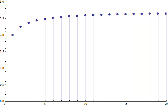
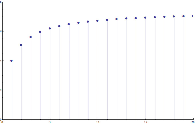
上式这个极限的值是连续情况下 $\lim_{x\to\infty}\left(1+r/x \right )^x$ 的一个子集，毕竟n只能为整数，而x为连续的值，可以为小数也可以为整数。所以我们可以选择不同的子集，只要保证最终的极限值是同一个。为了选择一个离散的子集，我们没有按照以前的习惯把r依次分布在1,2,3,4,5,6……份，即n依次为1,2,3,4,5,6……，而是把r平均分成rm份，其中m为整数，即n依次为1r,2r,3r,4r,5r……等等

Below is an example with r=2, to show that this procedure works (ie that our new limit will be the same as our old limit).

下方时r=2时的例子

The first plot here is of the sequence $(1+2/n)^n$

下方的散点图画的是序列 $(1+2/n)^n$

This next plot is the continuous limit $(1+2/x)^x$ , which is just a "filling in" of the discrete plot above by a continuous curve

下方的图是 $(1+2/x)^x$ 的图像，就像是把上方散点图之间的空白填充进去一样。

To make the limit easier to evaluate, we will select a different set of points from this original curve. Instead of evaluating at the original integer points, we will choose to evaluate it at the every even integer....ignoring every even point (此处应当是原作者笔误吧，既然选择了偶数点，那忽略的肯定是奇数点）effectively just compresses the plot by a factor of 2; but dosen't change the limiting value at infinity. As you can see, this new subsequence also tends towards the same limit (which happens to be e²).

为了让极限值比较好估计，我们从上图中选择不同的系列点。我们选择偶数点，忽略奇数点，就将这个图压缩了2倍。但是并没有改变无穷远处的极限值。正如你所看到的，我们选中的序列在无穷远处逼近e²

This procedure is carried out symbolically below, and allows for an actual evaluation of our limit:

这个操作的过程用符号表示如下所示：

$\lim_{n\to\infty}\left(1+\frac{r}{n} \right )^n=\lim_{x\to\infty}\left(1+\frac{r}{x} \right )^x=\lim_{m\to\infty}\left(1+\frac{r}{r\cdot m} \right )^{r\cdot m}$

Simplifying this last expression;

把做后一个式子简化得到

$\lim_{m\to\infty}\left(1+\frac{r}{r\cdot m} \right )^{r\cdot m}=\left[\lim_{m\to\infty}\left(1+\frac{1}{ m} \right )^{ m} \right ]^r=e^r$

Because we know that the limit within the square braces simply goes to e (by definition). Although it was a lot of work to reach this step; it was well worth it. This provides possibly the single most compelling reason that e shows up everywhere: it is not only the base representing 100% continuous growth, but continuous growth at any rate can be represented simply in terms of it, by simply raising e to the power of that rate! Out of all possible exponential bases, e is the only one with this property. It definitely makes sense to call e the "natural" base.

因为我们知道上式方括号中的值为e。尽管我们一步一步推导到此处花了很多时间，但这是值得的。这个推导过程是一个让人信服得理由，让人们相信e无处不在。e不仅仅代表100%连续增长率，而是任意连续增长率都可以用e来表示，只需要e的指数用该增长率替代就可以了。在所有的指数函数的底数中，e是唯一有这个性质的。（是吗？译者表示怀疑，哈哈）。那么此时称呼e为"自然数"就很自然而然了。

Before we talked about how via stretching any exponential could be written in terms of any other. Back then we didn't have any special exponential in mind, but possessing e now makes this property especially relevant. Given some arbritrary expoential; we know it can be written as a horizontal and vertical stretch of $e^x$ , so let's try and assign an interpretation to these stretches. Say for the two stretch factors a,b we are able to write our exponential in the form

之前我们讨论过如何通过伸缩变换将一个指数函数转化为底数不同的指数函数。但彼时我们内心并没有一个特殊的指数函数，现在我们可以用e作为这特殊的指数函数。对于任意一个指数函数，我们知道他可以写作经过横向拉伸和纵向拉伸之后的 $e^x$ 。那么我们现在尝试一下该怎么做。假设我们所要做的两个操作在公示中用a b来表示，如下，其中a表示纵向的伸缩变化。b代表横向的伸缩变化（前面有讲为什么）

$a\cdot e^{b\cdot t}$

Looking at t=0, we note the value of this exponential is simply a (this follows from the property that e⁰, or the product of no e's , is 1 as discussed before). Thus, the vertical stretch is equal to the amount at t=0, which we will call the initial amount. Also, by the properties of exponents we can see that

$e^{b\cdot t}=\left(e^b \right )^t$

And so b is simply the rate of continuous growth of our exponential. This gives us a nice intuitive picture of our exponential:

$a\cdot e^{b\cdot t}=(initial\; value)\cdot \left[ e^{rate}\right]^t$

Even more useful is this interpretation in reverse: say you want to encode mathematically the concept of starting with P of something which grows continuously at rate r. We can take the above expression and immediately write down our formula

$P\cdot e^{r\cdot t}$

Hopefully this discussion has left you with some reasoning behind the mantra "e is a special number". We can view e as the base of the function which equals its own derivative, as the maximal value attained by 100% growth distributed over the unit interval, or as the unit common to all continually growing processes. However, these properties still do not exhaust the usefulness of e: we will see below what the consequences of its simple differentiation formula are.

Differentiation of exponentials

It is again due to the properties of e that we have such simple formulas for the derivatives and integrals of an exponential function. The simplest case of course, is just that of $e^x$ , where we have the nice formula

$\frac{\mathrm{d} }{\mathrm{d} x}e^x=e^x$

Because all exponentials can be written simply as stretched copies of this curve, we need not even consider how to differentiate them individually. Instead, we can just focus on the derivative of $a\cdot e^{b\cdot x}$ , knowing that we can determining the appropriate values of the constants using some of our previous arguments. This is of course nothing more than a simple exercise of the chain rule; but we will try and go about it somewhat differently to develop some intuition.

The derivative of a function measures it's rate of change in the vertical with respect to the horizontal (thus the notation dy/dx), so the effect of a vertical stretch is simple to understand. If we multiply a function by a constant a, then we have replaced the y coordinate of each point on the graph with a point a times farther from the x-axis, but we have left the x coordinate unchanged.

If we view the derivative as the change in y relative to the change in x, we note that y changes a times as fast as before, whereas x changes at the same rate. Thus we would expect the change of our new function to be a times greater than before. In symbols; this is one of the properties that makes the derivative a linear operator:

$\frac{\mathrm{d} }{\mathrm{d} x}\left[a\cdot f(x) \right ]=a\cdot \frac{\mathrm{d} }{\mathrm{d} x}f(x)$

In the case of our exponentials, a vertical stretch equates to starting with a different initial amount. The above property can then be interpreted as saying that starting with an amount a causes the rate of change of your function to be a times greater than before. This makes perfect sense in our scheme due to the already-noted fact that exponential growth is characterized by the growth being proportional to the amount available. Since there is a times as much stuff, then it grows a times as quickly.

Now what about a horizontal stretch? Going back to thinking of the derivative as a limit of the ratio "y-change to x-change", we can see that a horizontal stretch leaves the y-coordinate unchanged, but stretches the x-coordinate. If we compress the x-coordinate by a factor of 2, then all of the y-coordinates will be brought twice as close together: that is our x-interval will be half the size that it was before the compression.

Because we are looking at the ratio y-change to x-change, if we fix our y-change to be the same, then our x-change is half of what it was, and the ratio is doubled (there was a 1/2 in the denominator). In general, if we stretch our x axis by a factor of b, then for the same y-change, we have an x-interval which is 1/b as large; making our new ratio b times the old. In symbols; this is the chain rule for constant coefficients:

$\frac{\mathrm{d} }{\mathrm{d} x}\left[f(b\cdot x) \right ]=b\cdot \frac{\mathrm{d} }{\mathrm{d} x}f(b\cdot x)$

Let's apply this reasoning to exponentials: a horizontal stretch of magnitude b is equivalent to a change of base in general. However, if we choose the base e to begin with, then a horizontal stretch of b can be re-interpreted as the rate of continuous growth. Applying the above rule for the natural exponential

$\frac{\mathrm{d} }{\mathrm{d} x}e^{b\cdot x}=b\cdot e^{b\cdot x}$

This simply says that if something is continuously growing at rate b, then its growth at time t is equal to that rate times the amount currently available. Evaluating this at t=0 provides an even simpler formulation

$\frac{\mathrm{d} }{\mathrm{d} x}_{x=0}e^{b\cdot x}=b$

which just states the obvious; if something is growing continuously at rate b, then when you have 1 unit of it, that unit is growing at rate b. Exponentials are so much simpler to work with once a nice interpretation has been constructed!

From this we can construct a formulation for the derivative of a general exponential $a^x$ : a simple horizontal stretch will allow us to write this exponential with base e. As was discussed before, the inverse function of e^x will provide us with the correct stretch.

$a^x=e^{\log_{e}(a)\cdot x}$

To stick with standard notation, we will denote the inverse of e^x as ln(x) from now on. This provides us with useful information even beyond just the ability to take the derivative, saying that something grows at rate $a^x$ is the same as saying it grows with rate ln(a). This interpretation of all different exponential bases simply being horizontal stretches of the natural base also gives us the following form of their derivative

$\frac{\mathrm{d}}{\mathrm{d} x}a^x=\frac{\mathrm{d}}{\mathrm{d} x}e^{\ln(a)\cdot x}=\ln(a)\cdot e^{\ln(a)\cdot x}=\ln(a)\cdot a^x$

which just says the rate of change is the growth rate times the current amount.

Computationally, one of the main advantages of e^x lines in the fact that it is its own derivative. From this its easy to see that the second derivative of e^x is also itself, as is the 3rd or any higher derivative. Most notably, every derivative takes the value 1 at x=0. To see why this is useful, consider the taylor series of a general function f(x). If f is analytic, we can express it in the form

$f(x)=\sum _{n=0}^{\infty}a_n\cdot x^n$

where the coefficients a_n are of the form

$a_n=\frac{f^{(n)}(0)}{n!}$

Using the fact that f⁽ⁿ⁾(0)=1 for all n, we see that e^xis the function with the simplest taylor series:

$e^x=\sum_{n=0}^{\infty}\frac{x^n}{n!}$

The plot below shows the convergence of the first 4 terms in this series towards the exponential:

This provides us with yet another means of calculating the value of e; one that turns out to be quite efficient: setting x to 1 in the above formula yields

$e=\sum_{n=0}^{\infty}\frac{1}{n!}$

which is much simpler to compute than the previous limiting definitions. A plot of the convergence of this series is below

Although more difficult to think about intuitively, this Taylor Series may be taken as the definition of e^x if you like. In fact, it is one of the most useful definitions to keep around, because it is easy to extend the meaning of the exponential to other domains, (e.g. what does e to the power of a matrix mean? e to a differential operator? e to the imaginary unit?) but we wont deal with it much here, extending the domain of the exponential via the approach "plug it into the taylor series and see what comes out" doesn't really provide much intuition behind why the extension behaves the way it does.

Imaginary exponents

指数为虚数

Without question the mainstay of electrical engineering, e with an "imaginary" exponent pops up everywhere: quantum theory, circuits, and even theoretical mathematics. The notion of e to a complex power should raise some flags upon first encountering it; much like before we extended the exponential from the integers to the reals, the expression doesn't mean anything until we assign it a definition and interpretation. We will start here by discussing the exponential eⁱ, and from that build up to an interpretation of more complex forms like $a^{(b+c\cdot i)\cdot x}$ or $i^x$ .

e的指数函数中指数为虚数，这在电气工程中非常常见，在量子力学，电路和理论数学中也能经常见到。第一次遇见e为底数指数为复数这种记号形式都会觉得奇怪，就好像我们之前在将指数拓展到实数范围时，如果我们不给定义，那么指数为某个实数这种记号形式本身并不代表任何意义。我们将从eⁱ开始我们的讨论，从而慢慢构筑指数为更复杂的复数记号形式的解释，比如 $a^{(b+c\cdot i)\cdot x}$ 这种形式或者 $i^x$ 这种形式.

Before delving into this, a quick description of the imaginary unit, i, is required. It is usually defined to be $\sqrt{-1}$ , and thought of as "imaginary" because this value does not exist on the standard number line. Here I am going to advocate a different interpretation of i, and of complex numbers in general, which will hopefully make them not seem so "imaginary" after all. The set of all complex numbers is often called the complex plane, and for a very good reason: a complex number can be written in the form

在深入探讨之前，我们对虚数单位i 快速回顾一下。一般把i 定义为 $\sqrt{-1}$ ，并把它称之为“想象的”[不太理解为什么翻译成“虚数”]因为这个值在实数线上是不可能存在的。这里我倡导一种不同的对于虚数i 和复数的解释，希望这种解释可以使得对于他们的理解不再“虚”，不再“想象中”。所有的复数集合被称之为复数平面。复数可以写成如下形式：

$a+b\cdot i$

a和b为两个实数

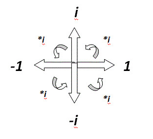
for two real numbers a, and b. We can identify this complex number with the point (a,b) on the plane, which lets us think of the standard x axis as the "real" axis, and the y axis as the "imaginary" axis. Just like the points in the plane, we can think of complex numbers as being a part of a vector space (meaning we can add them), but the complex plane has an additional structure of multiplication as well. Multiplication by a real number just corresponds to a "stretch" of the complex number, but multiplication by i actually represents a 90^o rotation. Lets look at a few examples:

a和b为两个实数。我们可以通过一组坐标点 (a,b)来在复数平面上确定一个复数，这就意味着我们把x轴是做“真实”，y轴视作“想象”。就像平面上的点一样，我们可以认为复数是向量空间的一部分（因为我们可以像向量加减法那样操作），但是复数平面有额外的乘法构造。一个复数乘以一个实数相当于对这个复数的“伸缩”，但是乘以复数i 相当于旋转90°。让我们看一些例子：

$1\cdot i=i$

If we view 1 as the vector of unit length on the horizontal axis, then multiplying it by i is the same as rotating it 90^o, which would line it up with the unit vector on the y-axis, the imaginary unit i.

如果我们把1看做x轴上一个单位长度的向量，然后1乘以i 意味着旋转90°，就变成了把他竖起来成为y轴上的向量，即为虚数的单位向量i 。

$i\cdot i=-1$

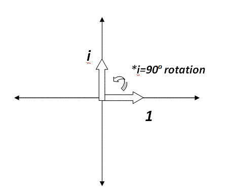上图中*i表示“乘以i”，*i=90° rotation表示“乘以i等价于90°的旋转”

This is the equation which has given i its interpretation as the square root of -1. A more useful interpretation of this is however that starting with 1, rotating by 90 degrees places it vertically on the y-axis, and another 90 degree rotation forces it to lie back on the x-axis, but pointing to the left. This more geometric interpretation is shown below

我们把虚数i定义为 $\sqrt{-1}$ ，上面这个式子就是虚数i 这么定义的来源。一个比较有用的解释是，从1开始，旋转90°向量变成y轴上的竖直向量，再旋转90°就变成了躺倒在x轴上且指向左边的向量。用图形表示如下图：

From this view of i, we can construct a meaningful interpretation for the expression $i^n$ : It represents n successive 90 degree rotations, or a total rotation of $n\cdot \pi/2$ radians. The cyclic nature of this function, cycling through the values {1,i, -1, -i} is shown below.

从这个角度来看待虚数i ，我们可以对表达式 $i^n$ 赋予一个有实际意义的解释。即为这个表达式代表了n次连续的旋转，每次旋转90°，或者说这个表达式代表了共计 $n\cdot \pi/2$ 弧度的旋转。这个函数的值在{1,i, -1, -i} 循环变化，示意图如下图：

We now have enough background to discuss what it means to raise something to an imaginary power. Looking at our previous interpretation of the exponential, eⁱ would represent the result of growing at rate i for one time unit. The fact that this does not make much sense at all is ok, we have simply moved our problem from figuring out what eⁱ means to what it means to grow continuously at rate i. Since i is simply a rotation, we may guess that "growing at rate i" may really mean "rotating," but to put any faith in this guess we will need some sort of proof. For this, we will go back to our definition of e^r as the limit of dividing a growth rate of r over the unit interval

现在我们有了足够多的背景知识来讨论指数函数中当指数为虚数时意味着什么。看看我们之前对于指数函数是如何解释的，eⁱ 表示会按照单位时间生长速率为i 来生长。这样来解释似乎没什么用，怎么解释不重要，我们现在通过这个解释将问题“eⁱ 是什么意思”转化成了问题“按照速率i 连续增长是什么含义”因为i 表示旋转，我们也许会猜“按照速率i 旋转”也许意思是“旋转”，为了让这种猜想更踏实一点，我们需要一些证据。我们需要回顾一下对于e^r 是如何定义的，我们把e^r 定义为把生长速率r均匀的分配在单位时间段内，将这段时间分的越细致，细致到极限。[这个翻译好难，后面我再改]

$e^r=\lim_{n\to\infty}\left(1+\frac{r}{n} \right )^n$

But this time, we will let the growth "rate" be a 90 degree rotation: i. For now, we will set this as our definition of what eⁱ means, and see if it has any useful properties.

但是现在我们令增长率为90°旋转。现在我们把这个定义为eⁱ的含义

$e^i=\lim_{n\to\infty}\left(1+\frac{i}{n} \right )^n$

Like before, we will try to gain some intuition by looking at the finite cases, on the way to the limit. For, say n=5, this can be written

就像之前那样，我们试着从有限的案例下得到一些直观上的概念和印象，比如当n=5的时候。

$e^i \approx \left(1+\frac{i}{5} \right )\cdot\left(1+\frac{i}{5} \right )\cdot\left(1+\frac{i}{5} \right )\cdot\left(1+\frac{i}{5} \right )\cdot\left(1+\frac{i}{5} \right )\cdot 1$

Where we can think of each of the quantities in parentheses as a set of "directions" for what to do to the vector 1. After the set, we have the new vector $1+i/5$ , which can be interpreted as leaving the vector 1 alone, and adding to it a copy of itself rotated by 90 degrees and shrunk by a factor of 5.

我们可以把括号中当做一个“方向”作用在向量(1,0)上，每次乘以括号中的部分，相当于旋转一个角度，这个角度就是括号中的部分所表示的。转动这个方向后，我们得到了向量 $1+i/5$ ，可以解释为向量(1,0)加上竖直方向的1/5的向量(1,0)

（关于这部分的理解，可以参考https://betterexplained.com http://jakwings.is-programmer.com/posts/29546.html http://www.360doc.com/content/18/0831/09/15509478_782614903.shtml 已经转载到了本作者所在的博客并标注了来源如果这里n=5不太理解，可以看看附录1中我写的matlab代码验证示例）

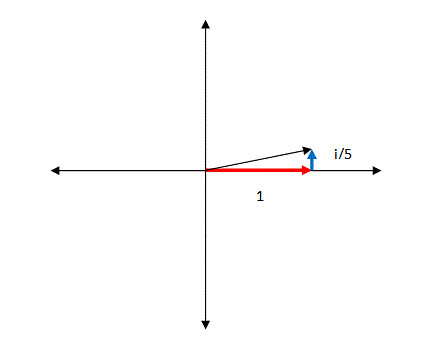Multiplying the second set of parentheses then takes this new vector as input, and adds to it a copy of itself rotated by 90 degrees and shrunk to 1/5th its normal length

乘以第二个括号中的部分意味着刚才产生的新向量作为输入，然后加入此时方向上的垂直90度1/5的新向量，如下图所示

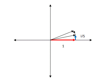Performing the next three sets of directions, we see the following picture emerge:

按照同样的步骤做完剩下的三步，我们看到下方的图

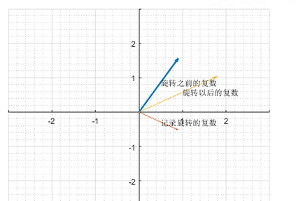
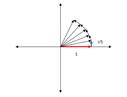Thus it appears there is something to our original guess that an imaginary exponent encodes rotation of some sort or another. In the above diagram, we see that the vector grows slightly in length with each rotation. However as we take larger and larger terms in the limit, the length increase is made smaller and smaller. In fact, in the limit, we start with the vector 1, and perform an infinitesimal rotation of it in the positive direction (by adding an "infinitely small" copy of itself rotated by 90 degrees), and then we repeat this over and over and over, slowly rotating the original vector more and more in the positive direction. What final value does our limit,

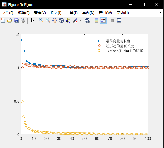
跟我们最初的想象类似，虚数代表着方向上的旋转。在上图中，我们发现每次旋转，向量的长度都会稍微增加一点，随着我们旋转的步数变的原来越多，每次旋转时增长的幅度也越来越小，比如我们旋转10次，每次旋转1/10的长度。当旋转的步数趋近于无穷时，我们从向量(1,0)开始，旋转无穷多次，每次正向旋转无穷多次分之一，旋转的角度为括号内的复数所表示的度数，如此这般旋转下去，慢慢的向着正向旋转。最终向量无限接近于哪个点呢？（参照附录2 我写的matlab代码记录最终的向量的长度）

$e^i=\lim_{n\to\infty}\left(1+\frac{i}{n} \right )^n$

converge to? We can calculate it numerically and see that it reaches the point (0.540302, 0.841471). The limiting path traced by the point on its way to its final destination is shown below.

我们可以计算出来，最终接近于(0.540302, 0.841471)。逼近极限的路径如下图所示：

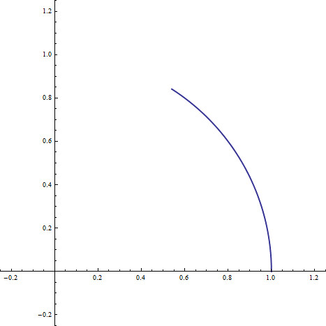While the specific coordinates of the point did not help us much understand what is going on, this picture is worth a thousand words. It turns out that the arc length above is exactly 1. That is, after unit time $e^i$ has moved exactly unit length along the circle. Thus, we were correct in guessing that imaginary exponents represented rotation, and even in this regime we find that e is a very special base: e is the base which represents rotation of unit speed when raised to an imaginary exponent. That is, not only is e the representation of 100% growth, but also of 100% rotation. What if we continue for t time units along this rotation path, instead of just 1? Since the point is traveling at unit speed, after t units it would have traversed a distance of t along the unit circle; or as we would usually say, the point would have been rotated by t radians. This allows us to assign a very intuitive picture to the commonly used expression $e^{i\cdot \theta}$ , it represents a rotation of $\theta$ radians.

得到最终指向点的坐标并不能帮助我们理解发生了什么，一图胜千言。可以证明这段曲线的长度为1.也就是说，进过单位时间 $e^i$ 旋转了单位长度。所以，假设虚数代表着旋转，那么此时按照这种思路走下去，我们发现e也是一个特殊的基底：e的虚数次方代表着旋转了单位长度的弧线。也就是说，e不仅代表这100%的连续增长率，也代表着100%的旋转。如果我们旋转t个时间单位呢？因为是按照单位时间旋转的，所以t个时间单位后会旋转t个单位长度的弧线。或者如我们所说，旋转了t个弧度。到此我们可以对经常用到的公式 $e^{i\cdot \theta}$ 有一个更为直观得理解，他代表着旋转了 $\theta$ 弧度。

If the base e represents rotation at unit speed, then what happens when we raise a different real number to an imaginary power? Just like in the previous cases, we are able to rewrite this new exponential in terms of e using the inverse function ln:

如果基底e代表着按照单位速度旋转，那么如果基底不是e而是别的实数会如何呢？就像之前的case，我们使用ln函数重写成如下形式：

$a^{i\cdot x}=e^{i\cdot \ln(a)\cdot x}$

After a unit time, this reaches the point $e^{i\cdot \ln(a)}$ , which from our above interpretation is just a rotation of ln(a) radians. Thus, the speed of rotation must be ln(a). Just as different bases represent horizontal stretches in the real numbers, they represent different rotational speeds in the imaginaries.

经过单位时间，到达了点 $e^{i\cdot \ln(a)}$ ，根据我们上面的解释，这其实就是旋转了ln(a)弧度。那么旋转的速度为ln(a)弧度每秒。正如上文中实数情况下基底的不同意味着水平的拉伸或者压缩，这里基底的不同意味着旋转速度的快慢。

We only have one more thing to discuss before we can fully interpret the imaginary exponential: what function the multiplicative constant out front has. Just like in the real case, we are able to write every imaginary exponential in the form for stretches in the independent and dependent coordinates.

在我们可以完全解释指数为虚数的函数形式之前，我们还剩一件事要讨论：如下式所示的常数r有什么用？（原文是out front在外边前边的 the multiplicative constant相乘的常数 what function 有什么用）。正如上面讨论的在实数范围内，我们可以把所有的虚数指数指数函数——就像下式的那种结构——写成不同坐标方向上的拉伸或者压缩

$r\cdot e^{i\cdot \omega\cdot t}$

We have already come up with a satisfactory interpretation for the constant preceding t: it is the rotational velocity (angular frequency) of the prescribed rotation, given in radians/time unit. What does the factor r do? Lets look at the case of t=0. Before r was introduced, the starting point of this function was the vector 1 in the complex plane. However, our new function has starting point r. Rotating this initial vector then at speed $\omega$ just traces out a circle of radius r, instead of the unit circle. The constant out front simply changes the radius of the circle on which the rotation is performed! This gives us a nice pictorial representation:

我们已经对于t前面的常数（即为小写omega，$ \omega $）有了一个比较合理的理解：这个$ \omega $的意义是旋转的角速率，单位是"弧度每单位时间长度"。那r是做什么用的呢？看下当t=0时的情况。在介绍r之前，$ e^{i\cdot \omega \cdot t} $这个函数的初始位置是复数平面上的向量（1,0）。然而我们的新函数 $ r\cdot e^{i\cdot \omega \cdot t} $的起始点为复数平面上的(r,0)。以角速度$ \omega $旋转这个初始向量得到的是半径为r的弧，而不是半径为单位长度的圆弧。式子外边的这个常数r只是改变了旋转运动的半径。那么当看到这个式子的时候就会有如下图景：

$r\cdot e^{i\cdot \omega \cdot t}=(radius)\cdot e^{i\cdot (velocity)\cdot (time)}$

$ r\cdot e^{i\cdot \omega \cdot t}=(旋转的半径)\cdot e^{i\cdot 旋转的角速度 \cdot 旋转的时间} $

Complex exponentials

We now have nice pictorial representations for exponentials with real or imaginary exponents. The most natural extension is to combine these; what happens if we have a complex exponent (one with both real and imaginary parts)? Because we can always write things in base e if we'd like to (and all of our interpretations are nicest in that base), we will write a general complex exponential as

$r\cdot e^{(a+b\cdot i)t}$

Before going through with this, we will look a bit at what is in the exponential to start with. In our original case of real exponents, the argument of the exponential was the real line (the input was of the form bt)

After that, we extended it to exponents of the form ibt, making the argument of the exponential be the imaginary axis of the complex plane

Now, we are attempting to use as an argument the term (a+bi)t, which is a general line in the complex plane through the origin with slope b/a:

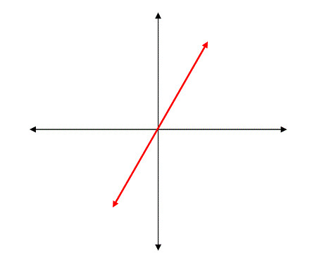If the real axis results in growth and the imaginary axis in rotation, what could exponentiating a line inbetween the two result in? If you guessed rotation and growth, you're on the right track! Lets try and put some rigor to this: looking at our above symbolic expression, we notice that we can use the laws of exponents to break the addition in the exponent into the product of two exponentials:

$r\cdot e^{(a+b\cdot i)t}=r\cdot e^{a\cdot t}\cdot e^{i\cdot b\cdot t}$

We have already assigned an interpretation to each of these terms, so understanding complex exponents is actually no problem at all: the r simply represents the length of our vector at t=0; the starting radius. The term $e^{a\cdot t}$ represents continuous growth at rate a, but here it is multiplied by the term $e^{i\cdot b\cdot t}$ which represents a rotation at angular speed b. Putting it all together, we have an initial radius of r which changes continously at rate a, while simultaneously rotating at speed b. To keep the spirit of the previous sections, we will write this out mathematically:

$r\cdot e^{(a+b\cdot i)\cdot t}=(initial \; raidus)e^{\left[ (rate\;of\;radial\;increase)+i\cdot(rate\;of\;rotation)\right ]\cdot (time)}$

Below is an animation of this process: it shows both the line in the complex plane which is taken as input, and the output of the exponential map. Note how when the line tends to the vertical (imaginary axis), the spiral limits in on the circle.

And heres the picture for initial radius=1, rate of growth=2, and rotation rate=3 (that is, the exponential map of the line with slope 3/2 through the origin of the complex plane)

Euler's formula

After all of the work we have done, the following may actually appear a rather trivial observation. However its usefulness cannot be overstated: Euler's formula is a connection of exponentials to trigonometry; in a way so simple and so elegant that one can translate between the two representations with ease. To see this connection, we will head back to the (hopefully now rather simple looking) e^it. This just represents rotation at unit speed about the unit circle, and looks something like this

At a given t, our unit speed point has moved t radians, which can be seen below

The expression e^itstands for this final position in the plane, but lets say instead of such a holistic view we would like an actual coordinate representation. That is, we would like to be able to write e^it=(a,b) for some a, b. Because the point (a,b) lies in the complex plane, we can also represent this point by the expression a+bi if we would like, but this is just a notational option, theres no real new information here. Lets look at what our coordinates would be. We know that the point e^it lies t radians away from the x axis, and that it lies on the unit circle. We can then use simple trigonometry to get the x and y projections

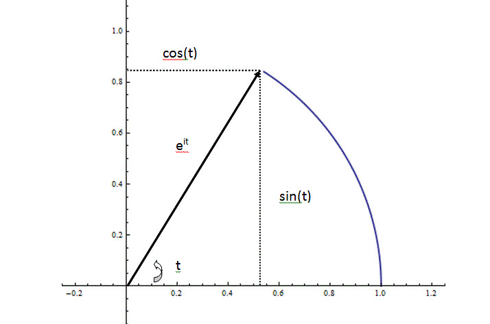This leaves us with the coordinate representation

$e^{i\cdot t}=(\cos t, \sin t)$

Which we can re-write as a point in the complex plane as follows:

$e^{i\cdot t}=\cos t +i\cdot \sin t$

Which is Euler's celebrated formula. This is simply an expression that continuous rotation at a unit speed (our definition of the symbol e^it) has a coordinate representation in terms of the trigonometric functions of the unit circle; which is nothing new. However take a step back, and forget all the interpretations and the work we have done so far; what this equation says is nothing short of amazing: the exponential function and the trigonometric functions were discovered independently, and their graphs look nothing alike. However it turns out that they are really one in the same. There is an over-reaching function on the complex plane such that when we restrict it to the real axis, we get growth, when we restrict it to the imaginary axis, we get oscillation, and all combinations of the two lie in-between. Rotation and exponential growth are two inseparable ideas, two faces of one function. Like space and time were fused by relativity theory into an immutable whole, growth and oscillation were by complex analysis.

The most well known use of Euler's formula is to show the rather startling identity

$e^{i\cdot \pi}+1=0$

This is simply a re-arrangement of the equation $e^{i\cdot \pi}=-1$ , which says that a rotation of $\pi$ radians simply moves 1 to -1. This is shown in the animation below:

When viewed as a statement about rotations, this is not very profound; again it is the form of the statement which is ridiculous. Here we have 5 very important numbers in mathematics: the additive identity, the multiplicative identity, the circle constant, the constant of rotation (i), and the natural exponential base; all related by 4 very important operations: exponentiation, multiplication, addition and equality. Whoa.

Summary of important properties

We've covered a ton of information here, so it's probably a good idea to highlight the important bits (plus, this will show you how far we've come!)

The "laws of exponents" themselves are just a consequence of our notational choice; namely "exponentiation is just a shorthand for repeated multiplication".

Negative exponents are a shorthand for repeated division

Reciprocal exponents (of the form 1/q) are another notation for the qth root.

Shifting an exponential horizontally is equivalent to vertically stretching it

Changing the base of an exponential is equivalent to horizontally stretching it

The unit base for discrete growth is 2.

The unit base for continuous growth is e

Starting with amount A and growing continuously at rate r is modeled by $A\cdot e^{r\cdot t}$

The exponential with base e is equal to its own derivative precisely because the proportionality constant between current amount and growth rate is 1.

While exponentiating the real line produces growth at unit rate, exponentiating the imaginary line produces rotation of unit speed

Exponentiating a general line in the complex plane results in radial growth and rotation simultaneously

The rotation produced by imaginary exponentials allows a nice useful connection to trigonometry.

Let me know if anything is confusing/what you think!

Steve

附录1：matlab示例，以下为matlab代码。为了验证任意复数a+bi乘以复数1+i/n后，如果把实部虚部当做向量的xy分量的话，那么旋转以后的向量长度为a+bi的长度乘以1+i/n的长度，旋转的角度就是a+bi原本的角度加上1+i/n的角度，从初始向量指向旋转以后的向量的这个向量与初始向量垂直。

clc
syms a b n real %matlab官方文档的解释 If you assign numeric values to these variables or specify that these variables are real, real can extract the real part of the expression:
%也就是说这里声明的变量a、b和n为real类型的，下面real()函数才能提取出来复数的实部和虚部
A=a+b*1i %A是旋转之前的复数
rotate=1+1/n*1i %rorate是用于旋转的复数旋转的角度，用复数来表示

B=collect(expand(A*rotate),1i) %B是旋转之后的复数 expand()函数是展开代数表达式，collect()类似于合并同类项，这里我指定将虚数i项相合并
from_A_to_B=B-A %C是从初始复数指向最终复数
A_vector=[real(A) imag(A)] %用平面内对的向量来代表平面内的复数初始复数所代表的的向量
B_vector=[real(B) imag(B)] %用平面内对的向量来代表平面内的复数旋转之后的复数所代表的的向量
ROTATE_vector=[real(rotate) imag(rotate)] %用平面内对的向量来代表平面内的复数 rotate=1+1/n*1i
from_A_to_B_vector=[real(from_A_to_B) imag(from_A_to_B)] %旋转完以后的复数所代表的向量 from_A_to_B=B-A
is_veticle=dot(A_vector,from_A_to_B_vector) %点乘为0，说明向量垂直

A_vector_length=norm(A_vector) %norm()函数是向量的长度
B_vector_length=norm(B_vector)
ROTATE_vector_length=norm(ROTATE_vector) %rotate=1+1/n*1i 的长度

from_A_to_B_vector_length=norm(from_A_to_B_vector) %from_A_to_B=B-A 是向量A长度的1/n

%下面是为了利用向量得方法求两个向量之间角的正余弦值
rotate_vector=[real(rotate) imag(rotate)]
i_vector=[1 0]

rotate_vector_3D=[real(rotate) imag(rotate) 0]
i_vector_3D=[1 0 0]
A_vector_3D=[real(A) imag(A) 0]
B_vector_3D=[real(B) imag(B) 0]

cosine_of_ROTATE_to_x_axes=dot(rotate_vector,i_vector)/(norm(rotate_vector)*norm(i_vector))
sine_of_ROTATE_to_x_axes=norm(cross(rotate_vector_3D,i_vector_3D))/(norm(rotate_vector_3D)*norm(i_vector_3D))

cosine_of_A_to_x_axes=dot(A_vector,i_vector)/(norm(A_vector)*norm(i_vector))
sine_of_A_to_x_axes=norm(cross(A_vector_3D,i_vector_3D))/(norm(A_vector_3D)*norm(i_vector_3D))

cosine_of_B_to_x_axes=dot(B_vector,i_vector)/(norm(B_vector)*norm(i_vector))
sine_of_B_to_x_axes=norm(cross(B_vector_3D,i_vector_3D))/(norm(B_vector_3D)*norm(i_vector_3D))

%和角公式计算A与x轴的夹角加上 rotate与x轴的夹角
cos_of_A_theta_plus_ROTATE_theta=(cosine_of_A_to_x_axes*cosine_of_ROTATE_to_x_axes-sine_of_A_to_x_axes*sine_of_ROTATE_to_x_axes) %应该与cosine_of_B_to_x_axes的值相等

sin_of_A_theta_plus_ROTATE_theta=(sine_of_A_to_x_axes*cosine_of_ROTATE_to_x_axes+cosine_of_A_to_x_axes*sine_of_ROTATE_to_x_axes) %应该与sine_of_B_to_x_axes的值相等

figure
axis([-3 3 -3 3])
grid on
grid minor
set(gca, 'XAxisLocation', 'origin')
set(gca, 'YAxisLocation', 'origin')
hold on

a=1 %测试的时候修改这三个数字就好啦
b=sqrt(3)
n=-sqrt(3)

A_substitue=subs(A) %subs()函数将代数里面的变量替换成实际的值
rotate_substitute=subs(rotate) %记录旋转信息的vector
from_A_to_B_substitute=subs(from_A_to_B) %B-A得到的vector
B_substitute=subs(B)

quiver(0,0,subs(real(A)),subs(imag(A)),'linewidth',2)
text(0.5*subs(real(A)), 0.5*subs(imag(A)),'旋转之前的复数') %text()函数在图中做标记前两个参数是做标记的位置，后面的字符串是标记的内容

quiver(0,0,subs(real(rotate)),subs(imag(rotate)))
text(0.5*subs(real(rotate)), 0.5*subs(imag(rotate)),'记录旋转的复数')

quiver(0,0,subs(real(B)),subs(imag(B)))
text(0.5*subs(real(B)), 0.5*subs(imag(B)),'旋转以后的复数')

length_of_A_vector=norm(subs(A_vector_length))
length_of_ROTATE_vector=norm(subs(ROTATE_vector_length))
length_of_B_vector=norm(subs(B_vector_length))

theta_of_A=subs(acosd(cosine_of_A_to_x_axes))
theta_of_ROTATE=subs(acosd(cosine_of_ROTATE_to_x_axes))
thete_of_B=subs(acosd(cosine_of_B_to_x_axes))
thete_of_A_theta_plus_ROTATE_theta=subs(acosd(cos_of_A_theta_plus_ROTATE_theta))

输出结果的一部分如下：

附录2 A向量一点一点旋转以后到最终的向量B处时最终向量的长度

n=20
a=1
b=0
A=a+b*1i %A是旋转之前的复数
rotate=1+1/n*1i ;

figure
axis([-0.5 2 -0.5 2]);
pbaspect([1 1 1]);
grid on
grid minor
set(gca, 'XAxisLocation', 'origin')
set(gca, 'YAxisLocation', 'origin')
hold on

quiver(0,0,1,0,'AutoScale','off','linewidth',5); %quiver()函数画向量，从0,0出发，向量为1,0 关掉AutoScale这样向量的头和尾部恰好落在坐标点上。向量的宽度linewidth为5
now_vector_length=[];
arc_length=0 %将每次移动的直线距离相加求和，得到的是连接历次旋转后的向量终点的线条的长度

position=1 %标示文字出现在要标示的向量的位置，单位是百分比
for index=1:n

if index==1
before_rotate=A;
B=A*rotate;
else
before_rotate=B;
B=B*rotate ; %B是旋转之后的复数
end


B_vector=[real(B) imag(B)] ; %用平面内对的向量来代表平面内的复数旋转之后的复数所代表的的向量
B_vector_length=norm(B_vector) ; %旋转以后B向量的长度
now_vector_length=[now_vector_length,B_vector_length] ; %数组用来记录历次旋转以后vector的长度，以数组形式记录

little_rotate=B-before_rotate; %little_rotate是一个复数，从旋转前的复数指向旋转后的复数
little_rotate_vector=[real(little_rotate) imag(little_rotate)]; %用平面内对的向量来代表平面内的复数这个变量是此次旋转的复数对应的向量
little_rotate_vector_length=norm(little_rotate_vector); %用平面内对的向量来代表平面内的复数这个变量是此次旋转的复数对应的向量的长度

quiver(real(before_rotate),imag(before_rotate),real(little_rotate),imag(little_rotate),'linewidth',2,'AutoScale','off')

%queiver()画向量，起始点为real(before_rotate),imag(before_rotate)点出发，画的向量为real(little_rotate),imag(little_rotate) 相当于在图中把旋转的向量给画出来了,并使用下面的代码标记这段为“每次旋转走过的直线长度”

show_position_x=(real(before_rotate)+real(B))/2;
show_position_y=(imag(before_rotate)+imag(B))/2;
txt_for_each_length = ['每次旋转走过的直线长度 ', num2str(little_rotate_vector_length)];

text(show_position_x,show_position_y, txt_for_each_length);
arc_length=arc_length+little_rotate_vector_length; %将每次旋转的小向量的长度累加

quiver(0,0,real(B),imag(B),'linewidth',2,'AutoScale','off'); %画出起始点在（0,0），向量为（real(B),imag(B)）的向量，向量的线宽为2 'AutoScale','off'这样显示向量就不会自动缩放了，向量的终点就会显示在正确的坐标位置上

txt = ['长度为 ', num2str(B_vector_length)]; %标记出此时一次旋转后向量B的向量
text(position*real(B), position*imag(B), txt)
end

figure('Name','旋转后向量长度的变化')
axis([-0.5 13 -0.5 2])
pbaspect([1 1 1])
grid on
grid minor
set(gca, 'XAxisLocation', 'origin')
set(gca, 'YAxisLocation', 'origin')
plot(now_vector_length) %画出向量在旋转过程中长度的变化

%我想看总共旋转的次数为1次（也就是rotate=1+1/1*1i ）， 2次（也就是rotate=1+1/2*1i ） 3次（也就是rotate=1+1/3*1i ） 4次（也就是rotate=1+1/4*1i ）等等到100次（也就是rotate=1+1/100*1i ），这100种情况下最终向量的长度是如何变化的，以及旋转所经过的路径总长度是如何变化的

可以看到，随着划分的越来越细，旋转的向量的长度几乎不变，经历过的圆弧的长度也无限趋近于1

m=100

a=1
b=0
A=a+b*1i %A是旋转之前的复数

record_of_last_vector_length=zeros(1,m); %1行m列的矩阵，并初始化为0 用来记录对应于m次旋转后最终向量的长度
record_of_last_arc_length2=zeros(1,m); %1行m列的矩阵，并初始化为0 用来记录对应于m次旋转后旋转向量的长度的累加值

record_of_difference_with_last_position=zeros(1,m); %1行m列的矩阵，并初始化为0 用来记录对应于m次旋转后旋转向量的位置距离根据欧拉公式得到的位置的距离

for index_out=1:m %1+1/m*1i中的m，平均分成几份，要转动几次
arc_length2=0; %arc_length2 随便起的名字，也可能叫arc_length3，arc_length4，等等，就是在当前m次旋转下，m次旋转向量的长度的累加值
rotate2=1+(1/index_out)*1i ; %1+1/m*1i中的m，平均分成几份，要转动几次这里i前面的数字对应于e的多少i次方，也对应于后面计算完以后接近于cos(1) sin(1)中的这个弧度，如果为rotate2=1+(1/index_out)*2i，那就是旋转完的复数末端点的坐标接近于cos(2) sin(2)
for index2=1:index_out %旋转index_out次
if index2==1
before_rotate2=A;
C=A*rotate2;
else
before_rotate2=C;
C=C*rotate2; %C是旋转之后的复数
end
little_rotate2=C-before_rotate2; %little_rotate是一个复数
little_rotate_vector2=[real(little_rotate2) imag(little_rotate2)];
little_rotate_vector_length2=norm(little_rotate_vector2);
arc_length2=arc_length2+little_rotate_vector_length2; %每次旋转走过的向量的长度都累加起来
end

arc_length2; %index_out旋转次数后走过的路程长
C_vector=[real(C) imag(C)] ; %旋转index_out次数之后的复数所代表的的向量

C_vector_length=norm(C_vector) ; %index_out旋转之后的复数所代表的的向量的长度

compare_of_last_vector_with_x_equal_cos1_y_equal_sin1=[(real(C)-cos(1)) (imag(C)-sin(1))]; %因为上边是rotate2=1+(1/index_out)*1i所以这里是与坐标点cos(1),sin(1)做比较
length_of_compare_of_last_vector_with_x_equal_cos1_y_equal_sin1=norm(compare_of_last_vector_with_x_equal_cos1_y_equal_sin1);

record_of_last_vector_length(index_out)=C_vector_length; %记录index_out旋转之后的复数所代表的的向量的长度
record_of_last_arc_length2(index_out)=arc_length2; %记录index_out旋转之后每次旋转的向量的长度的累加，即为累计所走过的长度

record_of_difference_with_last_position(index_out)=length_of_compare_of_last_vector_with_x_equal_cos1_y_equal_sin1; %记录index_out旋转之后最终向量的终点坐标距离预测坐标点cos(1),sin(1)的距离。因为上边是rotate2=1+(1/index_out)*1i所以这里是与坐标点cos(1),sin(1)做比较

end
figure('Name','细分不同次数经过的圆形长和最终vector的长度')
axis([-0.5 13 -0.5 2])
pbaspect([1 1 1])
grid on
grid minor
set(gca, 'XAxisLocation', 'origin')
set(gca, 'YAxisLocation', 'origin')
plot(record_of_last_vector_length,'s','DisplayName','最终向量的长度')
hold on
plot(record_of_last_arc_length2,'d','DisplayName','经历过的圆弧长度')

plot(record_of_difference_with_last_position,'o','DisplayName','与点cos(1),sin(1)的距离')

legend("show")

posted on 2021-05-28 14:15 无声烟雨阅读(488) 评论(2) 编辑收藏举报

刷新页面返回顶部

无声烟雨

[搬运]Exponentials: Discrete, Real, and Imaginary

Exponentials: Discrete, Real, and Imaginary

导航

公告