
[搬运]一篇讲傅里叶变换(Fourier transform)的好文章
国外的文章和教材有语言的障碍,但是没有理解的障碍;国内的文章和教材虽然没有语言的障碍,但是有理解的障碍。
有时间我会把其中比较关键的段落翻译一下,诸位共勉~
The Fourier Transform
傅里叶变换
|
The Fourier Transform and its inverse relate pairs of functions via the two formulas
傅里叶变换和逆变换可以用如下的一对函数来表示:
My goal here again isn't a rigorous derivation of these guys (this can be found all over the internet), but instead an explanation of why exactly they take this form, and what they do. The Fourier Transform is often described as taking a function in the "time-domain" and expressing it in the "frequency domain" (if the independent variable is time of course; above I used x but the formulas are the same regardless). To make sense of this notion, we will make a quick detour into vector spaces--don't worry, it will pay off in the end! We will use our review of vector spaces to motivate the notion that the Fourier Transform represents some sort of a "change of basis" for a function.
我并不是想要在这里严格的推导这两个公式(关于这两个公式的严格推导过程在互联网上到处都是),而是想要解释一下为什么这两个公式是这种形式,以及这两个公式是做什么用的。对于傅里叶变换的讲述经常是:将一个在时域的函数转换为一个在频域的函数(如果自变量是时间。上面的两个公式我是用x而没有用t来表示自变量,但是含义都是一样的)。为了使用这种形式表示出来的公式便于让人理解,我们快速复习一下向量空间——不要担心,等到最后会发现复习向量空间所花费的时间是值得的。通过复习我们会发现上面公式的表示形式其实是一种“改变基向量”的意思,只不过是针对函数改变的基向量而不是针对向量改变的基向量
Vectors and Bases
向量和基向量
To keep things simple, lets start out with a vector in
为了让事情简单一些,让我们从一个位于二维实数平面上的向量开始,我们把这个向量称之为v
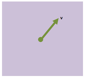 So far, we have no convenient way to express v, other than this picture. To help us understand v, lets bring in a set of basis vectors, vectors that are well-understood, and see if we cant write v in terms of them. Here, we choose to bring in the two standard basis vectors for
目前没有比用上面这张图更方便的方法来表示向量v。为了对向量v多一些理解,让我们引入一些基向量(对这些基向量我们有比较深刻的理解),看看能否用基向量来描述向量v。这里我们引入的是两个经常使用的基向量e1=(1,0), and e2=(0,1).如下图所示
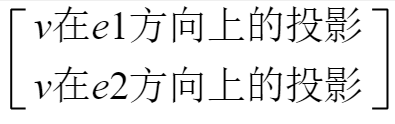
 To write v in terms of them, we need a way to somehow say "how much" of v is in the direction of each. Let's look at how to do this for e1. Let's say for a second we have a "projection" operation, which takes v and "squishes it down onto e1. We will call this
为了用基向量表达向量v,我们需要搞清楚v在其中任意一个基向量方向上走了多远。让我们看一下如何求出其在e1方向上走了多远。我们把这样的操作称之为投影,即为把v “压向”e1方向,看他在e1方向有多长。我们称之为
v在e1方向上的投影
 Now lets do the same for e2. We now have the "amount" of v in the direction of each of our basis vectors, so how do we go about using this information to describe the vector? Well, we used the projection operation and the basis to "take our vector apart", so let's put it back together! Multiplying each basis vector by the projection amount gives us two vectors, and adding these guys together gives us v back.
现在让我们用同样的方法求出 v在e2方向上的投影。现在我们知道了v在任何一个基向量方向上的投影长度。我们该如何用投影长度的信息描述向量v呢?嗯,就是通过在不同基向量上投影并将v在不同的基向量方向上分解。先用某个基向量方向的投影长度乘以该基向量,然后将他们相加,就得到了向量v
 In symbols;
用符号表示:
向量v=(v在e1方向上的投影)·e1+(v在e2方向上的投影)·e2
For now, we will do away with the projection notation, and simply refer to the components as the first and second components of v. That is, we will say that
现在我们会省略掉上面式子中的投影标记形式,而用简单的记号标记,表示形式如下:
If we already know the basis that is being used, we can even go a step farther towards simplification: we can label v by its two components alone! This allows us to "reconstruct" v at any time we'd like, because we could always just take the two components, multiply them by the respective basis vector, and add. This lets us say
如果我们已经知道所使用的基向量是什么,那么我们可以更进一步的简化记号标记,我们只需要用在基向量的投影来表示向量v。我们可以随时使用在基向量的投影乘以对应的基向量进而得到向量v。
v=
 现在,我们可以用坐标的形式来表示一个向量想,用来表示这个向量的坐标是我们通过将向量在不同的基向量投影之后得到的值。现在,如果我们在解决问题的过程中没有可以用来方便的解决问题的”标准的“基向量怎么办呢?我们会从不同的角度来审视向量v吗?我们一般都会选择一组新的基向量,比如下方的基向量
 (throughout this, we are only going to consider orthogonal bases, because that is all we will need to make the analogy with the Fourier Transform). We want a representation of our vector in terms of this basis? No problem; we can just project v onto each one like before
()一般类说我们只会考虑互相垂直的基向量,术语为正交的基向量,因为这是我们在做傅里叶变换的时候唯一需要做的。)我们想要用上方的新基向量来描述我们的向量v?完全没问题。跟之前的操作方法一样,我们只需要将向量v投影到两个新的基向量就可以了。
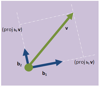 This lets us say
让我们来这样描述向量v
向量v=(v在b1方向上的投影)·b1+(v在b2方向上的投影)·b2
Which, if we know the basis, can again be shortened to
如果我们已经知道了基向量,我们可以简化对v向量的描述
v=
 Where the tildes represent the fact that now the components are the projections onto the b basis vectors instead of the e's. These two descriptions of our vector have different numerical values (as they should since each describes the vector in terms of the "amount" of it in a different direction), but there is no question they represent the same vector. From both representations it is simple to recover v, and in fact you can convert between the two representations with ease (think change of basis matrix).
v1上方的波浪符号表示这个值是向量v在b系列基向量上的投影而不是在e系列基向量上的投影。对向量v的两种描述值是不相同的,因为基向量不一样,所以投影应该也不一样,但是毫无疑问这两种表示方式都是指的同一个向量。从这两种表示方式中可以很简单的计算出向量v,并且也可以很容易的从这种表示形式转化为另外一种表示形式。(只要改变基向量就可以了)
Projections
投影
Let's take another quick detour and look at how to define the projection operator. We'll look at two vectors, u,v in
让我们快速的复习一下如何定义投影操作。加入现在实数平面上有两个向量u,v,如何定义向量v在向量u方向上的投影呢?
 If we look at this as a triangle, we know the length of the hypotenuse (its just |v|), and the projection we want is the length of the bottom side. If we know the angle between u and v; we can express this length as
如果我们看这个三角形,我们知道斜边的长度,也就是向量v的模|v|,向量v在向量u上的投影就是底边的长度。如果我们知道向量u和向量v的夹角,我们可以表示这个长度为:
向量v在向量u上的投影=向量v的长度 乘以 cosθ
This actually looks quite a bit like the geometric formulation of the dot product between two vectors. In fact;
这看起来就像是下方两个向量点乘的公式
And this lets us solve for the projection operator in terms of the dot product:
这样一来我们可以用点积来描述表示投影操作的记号(或者说投影运算的记号):
向量v在向量u上的投影=$ \frac{向量v点乘向量u}{向量u的长度} $
So, the projection of v onto u is simply their dot product, re-scaled by the length of u. If u is a unit vector then, the projection reduces directly to the dot product.
所以,向量v在向量u上的投影可以理解为向量v点乘向量u然后除以向量u的长度。如果向量u是一个单位向量,那么上面的投影计算式子就直接简化成了点积。
Dot Products
点积
It's time now to take a quick look at the dot product; but from now on we wont be restricting ourselves to
现在我们快速过一遍点积的知识。但是现在我们不会局限于实数平面上的向量。假设我们现在有两个向量,我们用基向量去描述这两个向量,即为我们可以用一系列数字的组合来表示这个向量。
向量v=$ \begin{bmatrix}
向量v在第1个基向量上的投影\\ 向量v在第2个基向量上的投影\\ ……\\ 向量v在第n个基向量上的投影 \end{bmatrix} $ 向量u=$ \begin{bmatrix}
向量u在第1个基向量上的投影\\ 向量u在第2个基向量上的投影\\ ……\\ 向量u在第n个基向量上的投影 \end{bmatrix} $ We can then express their dot product in terms of their coordinates:
我们可以用坐标的形式来表示向量u和向量v的点积:
$ \vec{u}\cdot \vec{v}=向量u在第1个基向量上的投影\times 向量v在第1个基向量上的投影+向量u在第2个基向量上的投影\times 向量v在第2个基向量上的投影+ ……+向量u在第n个基向量上的投影\times 向量v在第n个基向量上的投影= \sum_{i=1}^{n}向量u在第i个基向量上的投影\times 向量v在第i个基向量上的投影 $
So, in a coordinate representation, we can say that the dot product is the sum of the products of each coordinate. There is one more important point here: we obviously want this new definition of the dot product to agree with the geometric one; and if we allow our vectors to be complex numbers, to accomplish this we need to take the complex conjugate of one of our vectors, replacing the above with this new definition:
在坐标的表示形式下,我们可以说点积就是对应坐标乘积的和。这里有一个重要的点:我们显然想要这样的新的定义与几何层面上的相一致(请参考最后面附件解释1)。并且如果我们允许向量的坐标是复数,那么为了实现点积的坐标表示形式(即为“点积就是对应坐标乘积的和”这种形式),我们就需要将表示向量的坐标替换成原本数字的共轭复数
Where the overbar represents the complex conjugate. Obviously this definition reduces to the above if v has all real components, but the only important part is that this is the "good" definition, in that it agrees with our geometric definition, and allows us to use the dot product to express projections.
Just for the sake of having it for reference, lets look at how we would write out an n-dimensional vector in terms of projections onto a basis. For each basis vector, we would define a projection onto it, and this would give the "amount" of v in that direction. Our decomposition then looks like
The Fourier Transform
Whoo! Done with linear algebra! Time to try and make some sense out of the transform itself. Lets say we got some function f, whose graph is below:
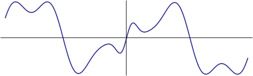 You can think of this graph as a "coordinate representation" of our function f. To each distance from the origin x, we can say the xth coordinate of f is f(x). We can picture this as being an infinite-dimensional analog of our vectors from before: just like for an n-dimensional vector, we can express it in terms of a basis using a list of n numbers, here we have an "infinite-dimensional vector" whose representation has an infinite number of coordinates, one for each x.
Now, the goal of the Fourier Transform is to decompose f into oscillations; which we can think of as analogous to our previous goal of decomposing v into its components along certain basis vectors. If we can accomplish this for f, then we can write f as a sum of frequencies: informally; if we let osc(k) represent an oscillation at frequency k, then (in analogy to the vector case above) we are looking to perform a decomposition of f of the form
Where fk represents the "amount" of frequency w in f(t). Our first order of business here is to decide how to model our sinusoids. We would like the sinusoid to be as "pure" as possible, because that way all of the useful information will be in the coefficient fk. As argued in Engineering Applications, complex exponentials form a very useful model for sinusoids, and a "pure" exponential of the form
 This allows us to make the definition
Also, the use of the summation sign here is merely suggestive; we need a formal way to "add up all the frequency components". The spectrum of possible frequencies is a continuous one (in our exponential above, k can take on any real number value), so we need some sort of "continuous" sum. Luckily, the integral is precisely that.
What we need now is a way to calculate the components of each frequency in the summation. Just like in the case of vectors, we would like to treat the modes of "pure oscillation" as our basis, and "project" onto them. The coefficient of each frequency would then just be the "amount" of it in the original function; and we'd be done. How could we go about this? Let's try and formulate something along the lines of our projection operator for vectors.
Just like we had
We are going to attempt to say that
So now, we just need to figure out how to perform this projection of f onto an oscillation. Previously, we were able to define the projection in terms of the dot product and a scaling factor, so let's go with that approach. But now, how are we to define a dot product of functions?
Again, lets take a quick detour back to our linear algebra analogy. We defined the dot product of two vectors to be
If we make a plot with the horizontal axis being the index (the value of i), we can represent this sum as just being the area of a bunch of rectangles added together, one for each index. For simplicity, lets draw the sum for the dot product of two 3D vectors:
  Visual representation of the dot product of two 18 dimensional vectors
 Visual representation of the dot product of two 100 dimensional vectors
 Visual representation of the dot product of two 1,000 dimensional vectors
How about for an infinite dimensional vector? Here, every single point on the horizontal axis represents a coordinate (the "xth coordinate of f"), and so we must sum over every coordinate -- over a continuum. Just like before, this continuous sum becomes an integral. Thus, like the dot product of vectors is the sum of the products of the coordinates; the dot product of functions (usually called the L2 inner product) is the integral of the products of the values:
 However, we do have one more thing to clean up. This definition works fine in the real case, but for complex functions we need to make sure to take the complex conjugate (again, this is to make sure that the dot product still works how we want it to; that it lets us define a projection operator).
Nice! Now we can try to piece together a definition of the projection operator we need:
The only ambigious part of this formula is the "size" of our oscillation function in the denominator. Since this is just a multiplicative constant in the formula, it's not really that big of a deal, but it turns out that if we set it to be
But, like for each projection,we need to divide each component frequency by
Where the amount of each frequency is given by
Look familiar? These are the formulas for the Fourier Transform and its inverse presented at the top of this post! The only difference between what we have here and the standard fomulation is the notation fk. To emphasize that there is a value of this for each real number k, the coefficients are usually written as a function of k, and to distinguish this function from f itself, it's given a hat:
Well, that was a lot of work (and a few detours!) just to get to these two formulas, but it was worth it. We can now make a quite precise statement about what each one says:
"A function f can be decomposed along a basis of oscillations and we can write f as a sum of those oscillations, weighted by how much each one contributes"
"The amount each oscillation contributes to f can be found by projecting f onto that particular oscillation"
The function holding all the contributions of each oscillation to f is called to Fourier Transform of f, and when you in turn take those components and use them to re-assemble f, it is called the inverse Fourier Transform. To make one more analogy to linear algebra, the Fourier Transform of a function is just the list of components of the function in the "frequency basis"; and the normal coordinate representation of the function is its expression in the coordinate basis.
We will usually use this standard notation to talk about the Fourier Transform from here on out to avoid confusion, but sometimes it will be useful to remember that the Fourier Transform is really just the formula for a projection, and the inverse is just a way of writing f in our new basis.
One important feature of the transform is that it is usually a complex function. While this may seem strange (especially if the input is real); its actually quite a natural thing. Remember, back when we chose the model for our oscillations, we decided to make it so that they all had 0 initial phase (that is, they are all cosines). So, if for some particular frequency k, the contribution to f is of magnitude 1/2 and initial phase of 45o, all of this information needs to be encoded into the coefficient
and thus, is a complex number. This shows us that the Fourier Transform at a particular frequency will be real if and only if that frequency contributes with an initial phase of 0, and complex in all other cases. In fact, when reasoning about the Fourier Transform, it will be easiest to express it in polar form:
In which A(k) is the amplitude with which frequency k contributes to f, and the exponential represents the initial phase (phase at the origin) of the contributing sinusoid. The "complex-ness" of the Fourier Transform isn't some magical property, but instead it's just a compact way to store both the magnitude and the phase of each contribution. The reason these are stored as complex numbers in our model is because we chose to use complex exponentials to model oscillation in the first place. We could of course have done this differently, keeping track of the amplitude and the phase of each contribution separately. But we wouldn't have ended up with something this nice :D
Visualization of the projection
We have already seen that the Fourier Transform is just a projection, but let's see if we can't find a way to also glean some insight into how this projection is accomplished. The formula for our projection tells us to multiply f by our desired oscillation, then to integrate over all x values. To make things a bit simpler; lets choose a particular frequency and just worry about that for the moment, say, frequency k. Our oscillation at frequency k is modeled by a complex exponential, which ammounts to a point rotating along the unit circle at angular speed k. Note that our required use of the complex conjugate in the projection actually makes this be a clockwise rotation:
 Now, we are told to multiply this by our function f(x). How do you multiply a function by a spinning dot? Well, it might first help to look at their product in symbol form:
Here we can see this is nothing but a complex number in polar form: the distance from the origin is given by f(x), and the angle by our exponential. As x varies, this represents a point spinning about the origin, but moving inward and outward according to the value of f.
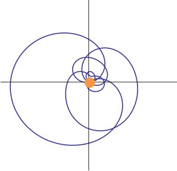
 As the complex exponential rotates, the function is "spun" about the origin
 The result of spinning a particular f at frequency 0.05
So, what does integrating this spinning thing do? An integral is just a continuous analog of addition, so in effect we are "adding together" all the points on the curve above. What does it mean to add these points? Well, they can be thought of as vectors (since the complex numbers form a vector space), so what we are really doing is adding together a bunch of vectors. At the end of the day after you've added a ton of vectors, what you are left with is the net effect of those vectors. You are left with a single vector which represents the action of all the other vectors "smashed together".
(ADDITION OF A BUNCH OF VECTORS)
(FINAL SUM=1 VECTOR)
Recap time: to calculate the projection of f onto a particular frequency oscillation, we first take f, and we spin it about the origin of a plane counterclockwise. We then proceed to find the average, or net effect, of all the vectors produced during the spinning. When we are done, we will be left with a single vector (or possibly nothing, if all of them cancel each other). This vector we are left with will have both an amplitude and a phase when viewed as a complex number, and these will represent the contribution of frequency k to our decomposition of f.
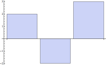
How could spinning a function at a certain speed manage to perform the projection we want? Lets look at an example to see. Lets say we define f as below:
I chose a function like this because it is quite easy to see "by inspection" what the component frequencies of it are. Lets say however, that we want to figure out how much the frequency 1 contributes to f. In standard notation, we are looking for
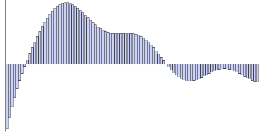
We will do this precisely by the method described above; we will rotate f in a circle at a frequency of 1, and then find the net effect. Because this particular function has a period of 2PI, there are some slight technicalities, but we can avoid them by actually just integrating over a single period1:
 Spinning the function at angular frequency 1
We can then take this plot, and treat each point as though it were a vector from the origin. Integrating over this curve then gives us the net contribution of frequency 1 in our signal. Below is a plot of the result of the spin, along with the normalized net contribution vector.
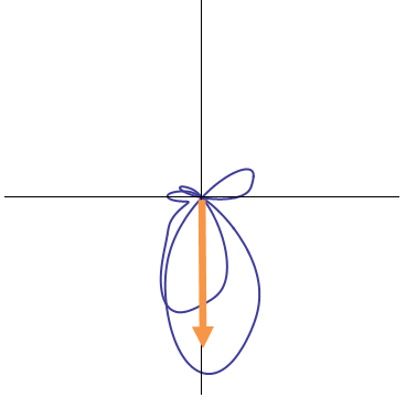 The net contribution of angular frequency 1 can then be seen to be represented by an arrow along the negative imaginary axis. The magnitude of this arrow tells us the amplitude of the contribution, and its phase (90o from the real axis) tells us that the contribution is sinusoidal.
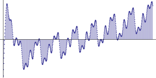
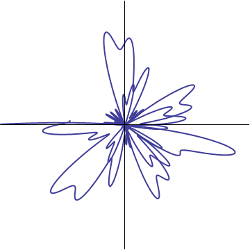
If sinusoidal contributions are represented by vectors along the imaginary axes, lets look at a cosinusoidal contribution: we will spin the function at an angular speed of 10 to single out the cosine at that frequency.
 Spinning the same function at angular speed 10
Although it is harder to see visually what the net contribution from this tangle will be, we can still perform the integral without difficulty. The rescaled net contribution is shown below.
 Thus, as we should have expected, the net effect is a smaller arrow along the real axis, representing zero initial phase.
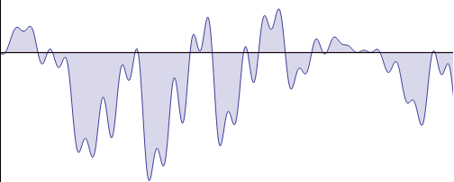
Yet another case we can investigate is that of angular speed 2. In our formula, we have both sinusoidal and cosinusoidal oscillations at that frequency. From elementary trigonometry we know that the sum of these two is a single oscillation with an initial phase shift. For illustrative purposes, let's perform our projection onto this frequency and see.
 Spinning the signal at angular frequency 2
Again, we can integrate this to find the net contribution of frequency 2:
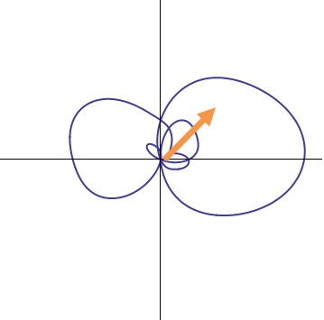 The net contribution is found to be phase shifted at 45o, representing a combination of both real (cosine) and imaginary (sine) components.
There's still one more thing we can check out with this example: what if we spin our function at angular frequency 4? Looking back at the original function, there is no oscillations at that frequency present; so we expect the Fourier component at that frequency to be 0.
 It turns out when we integrate this, the net contribution does go to zero! (A more formal way of saying theres "just as much" of the curve on each side of the origin).
 So, spinning a function at one of its "resonant frequencies" (a frequency that appears in it's spectrum) causes it to trace out a pattern from which information can be gleaned, whereas spinning a function at a frequency that it does not posess leads to random noise which in the end sums to zero. If the close analogies of the Fourier Transform with the projection function weren't enough to convince you that what we are doing here is "selecting" a frequency out of f, hopefully this short illustration of how the projection is accomplished is.
Abstracting the Transform
Well, we started with the goal of breaking a function apart into its component frequencies, and we were successful. Our treatment so far has not made obvious why instead of calling
Where we refer to the integral which performs the transform as
When viewed as an operator transforming functions into other functions, we also have another notation for the transform, which is sometimes more convienent. To express in symbols the idea "take the Fourier Transform of f" we write
Let's think about how we would write our notion that "a function can be written as a sum of its frequency components": well; its frequency components are encoded in it's Fourier Transform, and summing them together gets us right back to the original function itself. In operator-speak then, this amounts to the equation
Whats the use of doing this? Well, by itself its not that cool; but if you can find a way to translate not just functions, but entire problems using the Fourier Transform, it can give you a whole new perspective on the problem. Look at logarithms and exponentials. By themselves, they are just an example of a bijection of
Which is formally the same kind of relationship we have with the Fourier Transform and its inverse! This bijection dosen't just let us identify numbers in the two spaces however; it also lets us map operations back and forth. Namely, the rules of exponents tell us that the exponential of a sum is the product of the exponentials, and the log of a product is the sum of the logs. This lets us say
And through these two properties we can use the bijection to our advantage: if we have a sum that would be easier to understand as a product, we can take the exponential for a bit and just remember to take the logarithm at the end of the day. If we have a product that we would like to "break apart" with addition, we can use the logarithm, and then exponentiate later. In effect, the mapping of both numbers and operations between these two spaces gives us a "dictionary" of sorts, where given one problem we can translate it into a different, but equivelant problem which may be easier to solve. Also, although exponentiation originally had something to do with repeated multiplication, this is of no consequence here: all we care about is that there is some magic map (and inverse map) which lets us get new problems from old problems.
As we will see, this state of affairs is largely replicated in Fourier Analysis: we have constructed for ourselves a frequency decomposition of a function, but in the end this led to an abstract bijection between functions. Is there a way to make a "dictionary" between the two function spaces, like there is between the two number systems under exponentiation? It turns out there is; which is the main topic of Properties of the Fourier Transform.
Well, there's been a lot of jumping from one analogy to the next throughout this discussion, so its probably time for a good ole' summary.
Footnotes:
1: Using our formula, its clear that not all functions will have "nice" frequency spectra. Since the notion of projecting onto a frequency requires an integral over the entire real line, we need this integral to converge for it to be useful. Thinking about this requirement for a second; since our oscillation is made of a cosine and imaginary sine function; both of which are bounded in [-1, 1]; the magnitude of our integrand is going to be less than or equal to the magnitude of f at every point. If f is such a function that the integral of its square converges, then obviously the integral of f converges, and it follows that our projection integral (which is less than or equal to f's integral) must converge as well. We can formulate this requirement by saying that we only will allow ourselves to take the Fourier Transform of square integrable functions. You can go ahead and try to apply our projection formula to other functions, but what you get out won't itself be a function, but a more general distribution (like, the Dirac delta function or something). So; why is it ok to use the function in the example (which is obviously not square integrable) as an example? Think about the fact that after spinning one period of the function about the origin, we got an arrow giving the magnitude and direction of that frequency's contribution. If we tried to integrate over the whole real line (along which there are an infinite number of periods), we would get an infinite answer. If we did it carefully; we would get a delta function. Whats important here is that since each period is the same, all the useful information about the relative sizes and the phases of our eventual delta functions are contained within the spinning of a single period. Since this is all the information we were really after, I think it still holds as a valid illustration of the technique.
2: Before you can call it a bijection, you have to first identify functions with a finite number of removable discontinuities. This of course is a natural requirement, seeing that the transform is defined by an integral; and whatever values are taken by f on that set of measure zero aren't going to affect the integral's value.
附件解释1:
摘录如下:
|


 浙公网安备 33010602011771号