[搬运]关于卷积Convolution的一篇好文章
搬运自https://sites.google.com/site/butwhymath/m/convolution,这个博客一系列的文章都很好
国外的文章和教材有语言的障碍,但是没有理解的障碍;国内的文章和教材虽然没有语言的障碍,但是有理解的障碍。
有时间我会把其中比较关键的段落翻译一下,诸位共勉~
Convolution
|
Convolution is an operation which takes two functions as input, and produces a single function output (much like addition or multiplication of functions). The method of combining these functions is defined as
卷积是一种操作,用两个函数作为输入,产生一个单一的函数作为输出(很像加法或者函数的乘法)。合并这些函数的方法定义为如下表达式:
Where x, y both range over all of
其中x,y在$ \Omega $的所有范围内取值。在这里我会试着以解决某一个具体问题的方式来展示什么是卷积,然后再从中抽象出来卷积的数学概念和数学上的操作。
Propagation
传播
We will start our investigation by looking at some waves. Imagine you're standing on the edge of a pond, and you throw a small stone in. The stone will cause a ripple to travel outwards across the surface:
我们先开始观察一些波的扩散过程。想象你站在池塘边向池塘里扔一颗小石子,小石子会激起一圈圈的波纹。如下图所示:
 What about if the small stone was heavier? Well, intuitively we would expect a bigger ripple:
如果这个小石子更重一些会如何呢?哈哈,直观上来说石子激起的波纹会更大
 Or what about a lighter stone?
如果换成一个比较轻的石子呢?
 All three of the ripple patterns above share the same general shape, but differ only in their magnitude. How do we go about expressing this observation mathematically? First, let's abstract a bit: if we look at the impacting stone as our input, and the resulting ripple as our output, we then have a process to model:
上面三种不同大小的波纹都有着共同的形状,只不过强度不一样而已。我们如何用数学描述我们观察到的现象呢?首先,让我们做一点抽象。如果我们把投入湖中的石子当做输入,石子产生的波纹当做输出,那么我们就有了如下的描述这个过程的模型:
石头 ——>波纹
We can express the dependence of the ripple's size on the weight of the stone by saying that the output scales linearly with the input:
影响波纹大小的因素是石头的重量,我们可以把这种相关关系描述成输出与输入成线性关系,也就是说石头的重量增加一个比例,对应的波的强度也增加一个比例。
c*石头——>c*波纹
This property lets us see that there is some "special" stone we could study: that of unit weight. If we know the ripple caused by this stone, we can then find the ripple caused by any stone (lighter or heavier) by just scaling by the proper amount. If we think of this stone as appropriately "small" (technically, a point), then mathematically we can model it by an impulse. The wave caused by this unit weight pebble is called the impulse response, a relationship we can throw into symbols as follows:
这种性质使我们看到有一些“特殊”的石头我们可以好好研究一下,也就是单位重量的石头。如果我们知道单位重量的石头所激起的波纹,我们就能计算得到任意重量的石头所激起的波纹。只需要在前面乘以一个石头相对于单位重量的石头有多重就可以了。如果我们假设这个石头非常小(比如小到只有一个点的大小),那么数学的描述上我们就可以把他描述成一个脉冲,或者一个刺激。由这个脉冲所引发的波称之为针对单位脉冲的反馈。我们可以把这种关系用符号来描述,如下:
脉冲——>反馈
Where
在这个用符号描述的式子里,$ \delta $ 代指脉冲,而 $ h $代指一个系统接到单位脉冲时的反馈,在这个具体的例子里指代石头溅起的波纹。目前为止,知道单位脉冲的反馈h,我们就可以计算得到任何重量的石头所激起的不同强度的反馈,或者说波纹。那么我们还能做什么呢?哈哈,他说明了很多东西。比如说,目前为止我们都是把石头投入到原点(从数学上来说),但是完全可以预期无论把石头投向哪里,波纹的形状都一样。我们可以这样表述:如果我们平移脉冲的位置,那么我们也就平移了脉冲引起的反馈。用数学符号表示如下:
脉冲(位于某位置处)——>反馈(位于某位置处)
r表示原始位置,r0表示移动的方向和距离。脉冲往哪个方向移动,对应的反馈就往哪个方向移动。
What about if we drop two stones in at once, but at different locations?
如果我们同时扔进去两个石头呢?如下图
 The wave caused by two stones is just the sum of the waves produced by each stone. In math-speak:
两个石头所引起的波纹是每一个石头所激起的波纹简单的叠加。在数学上的描述为:
脉冲(位于位置1处)+脉冲(位于位置2处)——>反馈(位于位置1处)+反馈(位于位置2处)
Together with the scaling property we had from above; this lets us say our ripples are linear. To clear up notation from here on out; I'm going to replace the arrow with a function, w, so that instead of saying
再加上我们上面提到的反馈的强度是怎么样来变大或者缩小,我们就说波纹是线性的。为了从这里开始简化描述,我打算把箭头表示的关系替换成函数来表示,函数w,
We will say
Let's say now that we have a handful of small pebbles of all different weights. We throw them into the water and they spread out, impacting at all different locations. How are we to model the complex ripple that will result? Well, upon impact, the surface just experiences a sum of stones
And each stone can be viewed as a scaled and translated version of our unit stone (
 Now, what does the wave that results look like? We can just apply our "wave operator", w to the impact:
Which we can phrase more mathematically by
We are now in a position to use our previous knowledge of the linearity of our "wave operator" to write this more explicitly: we know the wave of a sum is the sum of waves, and the wave of a scalar multiple is the scaled wave of the impulse, so we can go ahead and express this symbolically
Now, we have expressed the resultant wave as just a scaled sum of various "unit waves", which we already have an expression for: h
Assuming we know the form of this function h then (the impulse response), we know the full form of our solution for the handful of pebbles:
 What have we learned here? Well, assuming we know what wave propagates from a unit impulse at the origin, we are able to figure out what the wave looks like for a collection of various impulses all over the place. Given a difficult problem (what does the water's surface look like when you throw a handful of pebbles in), we were able to reduce it to a much simpler problem (what happens when you apply a unit impulse at the origin), and the answer to this question and from it construct the answer to our original problem.
Where our evolution function w is both linear and translation-invariant (meaning we can break the input up as a sum of simpler parts if we'd like, and no matter where an impulse occurs the response looks the same). But what if our input isn't a simple sum of impulses? What if the input is a continuous function? Such a case could easily arrive in our wave analogy, if instead of dropping a pointlike pebble, we instead dropped in an extended object, like a cardboard box or a rock. If we would like to use the line of reasoning above, we need some way to break this complex input into impulses somehow:
If we can manage to do this, then we can solve our problem simply: we just need to apply w to each impulse individually, and sum the results!
To do this however, we are going to switch to a different physical analogy (don't worry, we will come back and solve the wave problem in a bit!). The reason for our switch-up is just to simplify the problem at hand: with waves we have to worry about the time dependence of our response as it travels through space, which doesn't affect the nature of the problem at all. After all, off in abstract-land all we are doing is dealing with problems of the form
Instead of water waves, lets say we are going to take a picture. The setup is something like this: an object to be photographed, the camera lens system, and a piece of film.
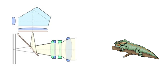 The goal of our camera is to take light from the original object and deposit it on the lens; so we can think of our camera as a function from object to film. If we call the object to be photographed the Source, the function to the image the Camera, and the film the Photograph, we can reduce this to a simpler schematic diagram.
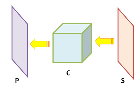 If we shine a bright light at the camera, we expect a bright image; if we shine a dim light, we expect a dim image. If we shine two lights, we expect two images. So, we can say that our camera function is linear, much like the waves. We can symbolize this relationship
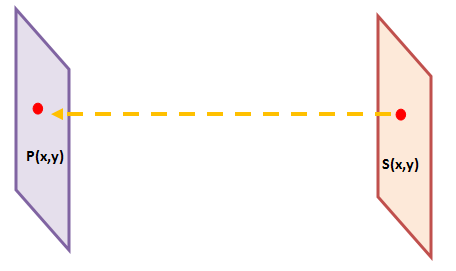
If our camera is in focus, we expect to see on the image exactly what what was around in the real world. That is, we expect a 1-1 correspondance between the source plane and the photograph.
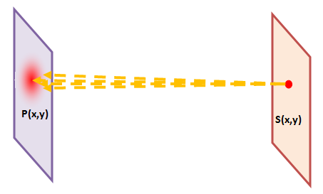
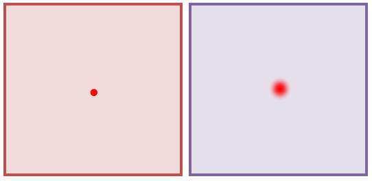
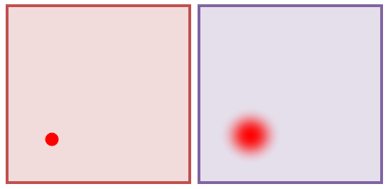
 What if our camera is out of focus? We know from experience that this means what appears to be a single point in the source (think a star) is a smudged blob on our photo. Thus, we don't have a 1-1 correspondence anymore, single source points spread their influence to multiple image points:
 In exact analogy with our wave example, lets say now we take our camera and image the night sky. The source plane (the cosmos) contains a multitude of stars, each of a different brightness. What will our image look like? Well, just knowing how a unit impulse at the origin is imaged, we can figure it out! Viewing each star as a stretched and translated unit impulse; our image will be a collection of stretched and translated blurs. We can decompose the night sky into a sum of these modified impulses, and then distribute our imaging function over the sum, blurring each star individually and adding the results.
 Symbolically say
Where mi is the brightness of each star, and (xi,yi) is its spatial location.
 Source Plane
If we want to determine what our photograph will look like, we can say
And again, we already know how C affects a unit impulse: it turns it into h! This gives us our solution:
 Photograph
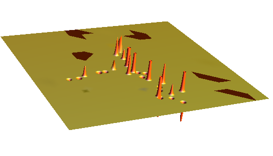
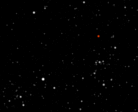
So far we have come up with two seemingly different problems; both which have a simple solution if we first understand how an "impulse" is propagated through them. Now lets take a picture of a portion of the sky with even more stars in it: for example, this small globular cluster which orbits our home galaxy:
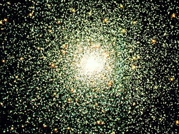 Source Plane
We can apply the exact same reasoning as above here: each star is like an impulse, so to see how each star will look on our final picture, we simply take that impulse, propagate it through the camera until it becomes our response function h, and then add all of them back together. The resulting blurry photo looks like this:
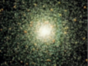 Photograph
It's time to make sure the mathematical formalism of this process really makes sense: at the location of each impulse (star), we apply our "blur" function which models our camera's lack of focus. This blur function spreads the light out from this original point source to a more extended region. If our star is located on the source plane at point (xi, yi), we need to make sure that our final image of the star is centered on that location as well. We defined our function h(x,y) to be the blur caused by a unit impulse at the origin, so we need to slide this impulse to occur at our new point (xi, yi) instead. This is what the term
  So far, this has just been a more careful repetition of what we have done above. What we are going to do now seems to be a simple change of symbols, but will actually give us some profound insight into convolution itself. The number mi represents the brightness of our ith star, which is located at the point (xi, yi) on the source plane. What this is really saying then is that the brightness of the source plane at location (xi, yi) is given by mi. That is, we can define a function on the source plane which gives us the brightness at each point. Lets call this function m(u,v). Given a point (u,v) of our source plane (the night sky), m tells us what the brightness is there. Of course, in our star examples so far most points of the plane have a brightness of zero (black sky). But as we saw in the globular cluster, if we try to image a part of the sky with lots and lots of stars, some of them will seem to touch, and form extended areas of brightness.
In fact, in the limit lets say we find a point of the night sky where there are stars everywhere. There are no dark points, every line of sight ends in a star. Our brightness function m would be nonzero everywhere, and every single point of the sky would have an impulse (star) located at it. Can we use what we have learned so far to figure out what our photograph of this area would look like? Sure we can! The only difference now is that we have a continuum of stars, instead of discrete points. But, at each location (u,v) in the night sky, we have an impulse with brightness m(u,v). We can represent this star by this brightness multiplied by an impulse function shifted to be located at (u,v):
This single point source dosen't propagate through our camera unchanged, however; it becomes blurred. This blur is still centered around the original location of the star however, and scaled for brightness by m(u,v) so we can say the image of this particular star is
Just like in our discrete cases above, we now just need to sum up the images of each star to get the final image. This sum needs to be taken over each (u,v) which has nonzero brightness, which in the present case is all of them! We will need to perform a continuous sum then, over each position (u,v).
This last equation just says the image of our continuous field of stars is the blurred image of each star individually, all added back together. However, this also happens to be a realization of the formula for convolution presented at the top of this post! The resulting image of our star field is just the convolution of our brightness field with the blurred image of a unit star at the origin!
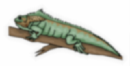
Since we already know how our camera responds to a unit impulse, all we have to do to model the photo of our lizard with the blurry camera is to take this response, scale it by the brightness at each location, and add them all up.
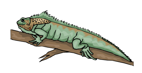  (It's probably time for a new camera!)
The blurry image is then just the convolution of our original image of the lizard (the brightness field), and the response of the camera to a single impulse.
Alright then, back to the water waves. What if we threw a larger object into the pond? Instead of having a discrete set of impulses to start the water vibrating, we have a continuous field of applied pressure.
(PRESSURE FIELD APPLIED TO WATER INITIALLY)
Just like with the image of the lizard, we can look at this contiuous field as simply being a bunch of scaled impulses smushed up next to eachother. To find the wave caused by this, we just need to find the wave caused by a single impulse, translate it, scale it, and add them all up
Again, we recognize this as a convolution of the wave caused by a single impulse and the pressure field of the extended object:
These two examples give us a bit of a feel for what convolution is. If we know how a certain system reacts to a simple impulse, we can figure out how that system reacts to anything, by first breaking it down into impulses, sending each through individually, and adding them up at the end. When we add them all up, we have to make sure to shift all the functions appropriately and scale them (so it matches up with the input) and taking care of this turns our sum into a convolution integral. Convolution is just the continuous analog of the problem solving strategy "break it down into small parts, solve those, and put em back together at the end".
Convolution seems to be a quite common operation throughout mathematics though; so let's see if we can find other places where it arises to further broaden our intuition.
Consider for a moment a metal rod which we have heated in some way. If we let it sit out, it will obviously cool down, but how do we express this quantitatively? Via a partial differential equation known aptly as the "heat equation", given the initial temperature of our rod (as a function of position), we can solve for its temperature at all future times.
For a general initial temperature distribution this may be a hard thing to do. So let's see if we can stick to the reasoning that's proved fruitful so far, and consider the effect one "impulse" of heat has on our rod. The mathematical model for this is
The solution to this problem is called the "fundamental solution", and can be visualized as follows:
 In this image, the red represents "hot" and the blue "cold". At t=0, we apply an impulse of heat to our rod (think of touching a soldering iron to it), and as time progresses that heat spreads out and evens out, as we would expect it to. We can alternatively choose to plot the heat distribution in a "standard" graph:
 Where the vertical dimension gives the temperature at position x.
Solving the heat equation analytically for this particular initial condition, we can arrive at a closed form of this fundamental solution (here we will take the constant to be unity)
The most important part however is not the form of this solution, but rather the form of the problem: the transformation of our initial impulse into a different function:
If we had decided to place the soldering iron at a different location than the origin, we would expect the same heat distribution to result, and so this process is translation invariant. Had we placed two soldering irons, we would expect the result to be the sum of two dispersing heat waves, and if we had placed a hotter iron, we would expect a hotter rod; the heat equation is linear and translation invariant.
In abstract-land, this problem is identical to both of the above. We have some sort of a correspondence between an impulse and a function, and we can write this correspondence in a linear, translation-invariant manner. Thus, we expect that if we heat the bar via some continuous distribution instead of an impulse, we can find the final solution to our problem by convoluting the initial temperature with the impulse response. As an example lets say we heat the bar to the right of the origin, and cool it to the left so that the initial temperature distribution looks something like this:
 Or, in symbols:
To solve for the temperature distribution caused by this initial condition, we will view f as being composed of a bunch of mini impulses, right next to eachother. Feeding each impulse through the heat equation will give us a shifted and translated version of our fundamental solution, and adding them all back together will give us the answer we seek. This is of course, just the convolution of the initial condition and the fundamental solution:
Since our initial condition is only nonzero over the finite range (-3,3), we can re-write this integral as
Performing this integral, we get
Which is much more easy to understand pictorally:
  We can see qualitatively that the temperature distribution tends to "smooth out" as time progresses, much as we would expect. This example provides some good mathematical justification for the use of convolution: in addition to it being intuitively simpler to break a problem into impulses and then just re-combine them, it's hard to see how to even come up with an analytic expression as complicated as the solution here if we had not first solved for the fundamental solution, and then gone used convolution formally to compute the desired answer.
There's one more type of problem where convolution is common in its solution:
To satisfy the first property, we must first understand what we mean by the "size" of a function. For our purposes we will say that size is equivalent to the area under that function; in symbols
By being point-like and centered at the origin, we mean that our impulse is pretty much zero at all other points. This fits well with our intuitive examples of impulses, the small pebbles and starlight. How could we go about constructing some function like this? For a starting place, look at the normal curve:
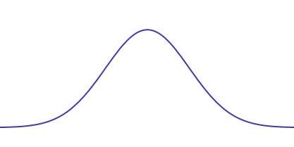 By construction this curve has a total integral of 1, and it's roughly concentrated about the origin. What can we do to make it more "point-like"? The following animation shows a sequence of normal curves (each of total integral 1) with increasingly small standard deviations.
 As the standard deviation decreases, the curve becomes more and more centered at the origin, which is precisely what we want. It appears that if we shrink the standard deviation towards zero, the curve will collapse onto the origin into one single, infinitely thin spike.
 Since all of the normal curves limiting towards this spike had area 1, we will say this spike has "area" 1 as well, it is the "unit" spike. This guy will serve us perfectly as a unit impulse.
However, this isn't the only way to define our impulse. What if instead of squishing normal curves towards the origin, we squished a unit square? As its base gets smaller and smaller, it must grow taller and taller (to preserve the unit area inside of it) and again in the limit we will end up with a spike-like object centered on the origin, which we can say has unit area. In fact, there are a bunch of different curves we could use in a limiting procedure like this, and our final notion of impulse is independent of that choice.
|