『论文笔记』Attention Is All You Need

一、论文简介

https://arxiv.org/abs/1706.03762

一篇外网博客，可视化理解transformer：http://jalammar.github.io/illustrated-transformer/

 A TensorFlow implementation of it is available as a part of the Tensor2Tensor package. Harvard’s NLP group created a guide annotating the paper with PyTorch implementation.

Follow-up works:

• Depthwise Separable Convolutions for Neural Machine Translation
• One Model To Learn Them All
• Discrete Autoencoders for Sequence Models
• Generating Wikipedia by Summarizing Long Sequences
• Image Transformer
• Training Tips for the Transformer Model
• Self-Attention with Relative Position Representations
• Fast Decoding in Sequence Models using Discrete Latent Variables
• Adafactor: Adaptive Learning Rates with Sublinear Memory Cost

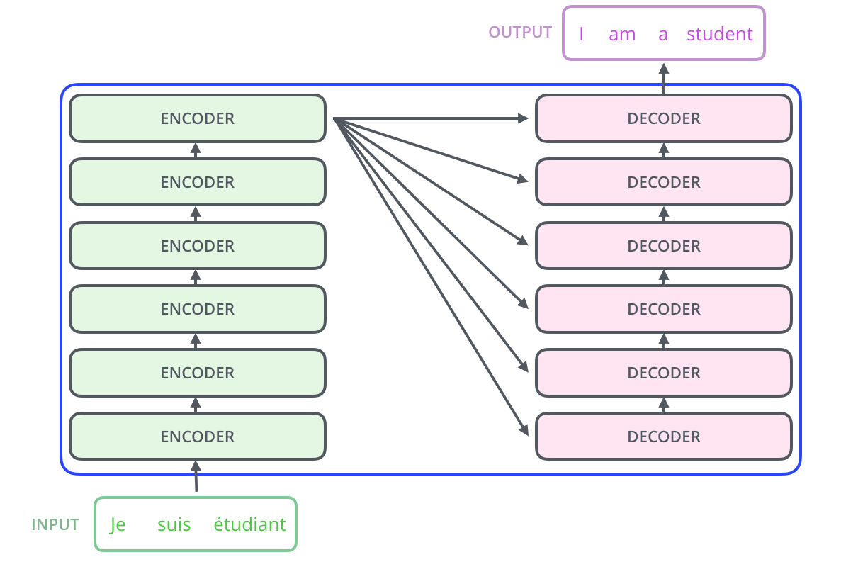
网络概览

二、自注意力机制

1、自注意力机制原理

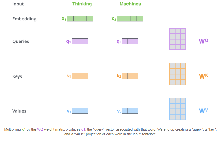
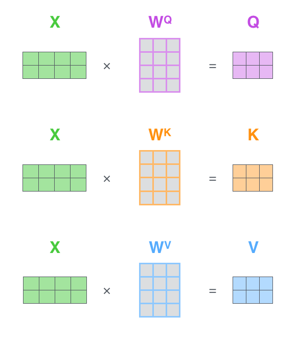
a、Embedding计算query、key、value向量

Embedding向量会分别经过三个矩阵生成三个向量，考虑到计算量，三个向量的维度大大小于Embedding（512->[64，64，64]）

b、词间相关度

词a的query向量和词b的key向量点乘作为两者的相关度得分

c、相关得分后处理

得分值除以8（向量维度64的平方根，原文默认的值，似乎没什么讲究），然后作SoftMax处理。

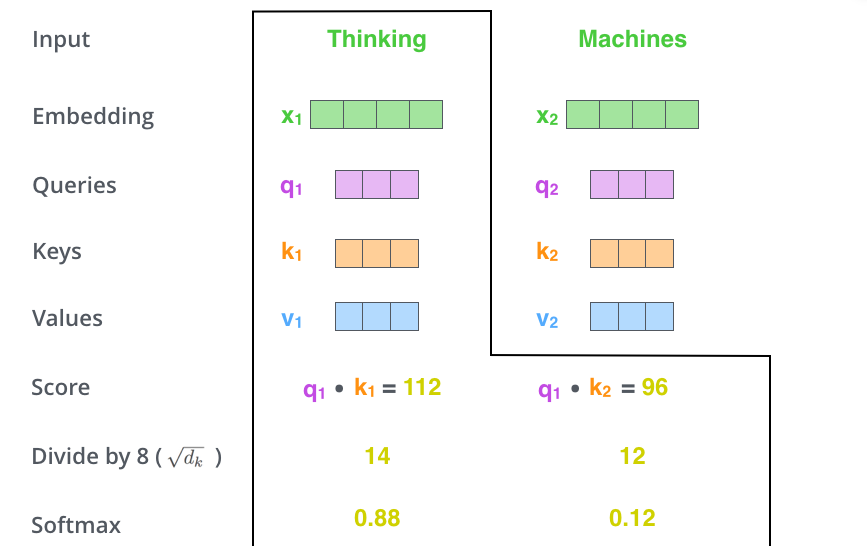
得分表示了当前位置将表达的含义和输入word们的相关性： 

This softmax score determines how much each word will be expressed at this position. 

 

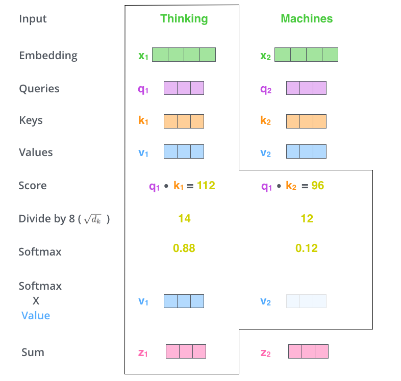
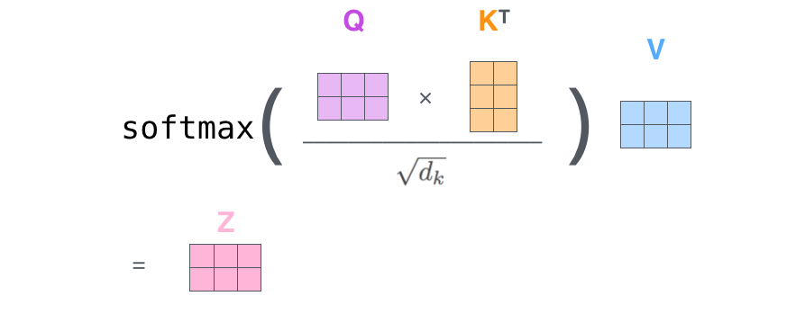
d、Self Attention输出

Self Attention在每个位置上将输入Embedding映射为一个新的向量。每个位置的输出为：在全部位置上对应的Values向量乘对应的SoftMax得分，结果进行sum（说起来比较绕，建议直接看下图）。

2、矩阵化自注意力机制加速

Q*K^T输出为n*n的矩阵，每个位置表示行列inx对应word的相关度。每一行对应上图中黄色数字的一行，这样Z的每一个元素即为V上每一列的加权和。

 

 

 

 

 

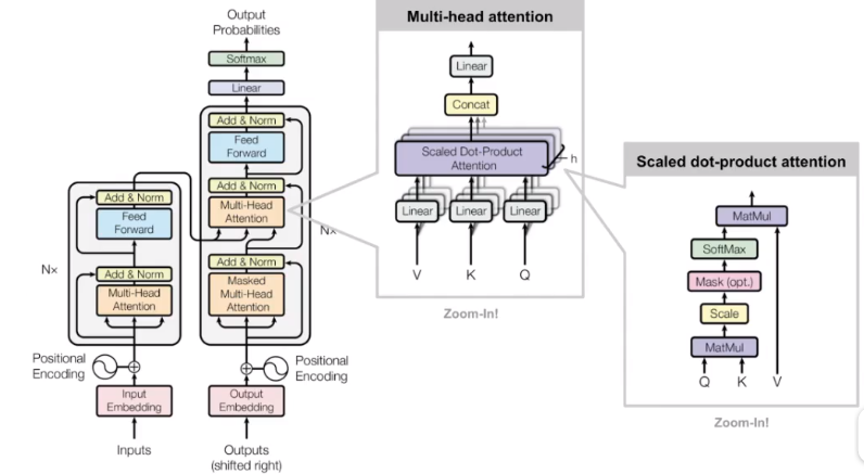
3、 多头注意力机制

文章进一步扩展了自注意力机制为多头注意力机制：使得一个位置可以关注多个相关位置；使得模型可以使用多个特征表示子空间。

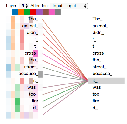
1. It expands the model’s ability to focus on different positions. Yes, in the example above, z1 contains a little bit of every other encoding, but it could be dominated by the the actual word itself. It would be useful if we’re translating a sentence like “The animal didn’t cross the street because it was too tired”, we would want to know which word “it” refers to.

2. It gives the attention layer multiple “representation subspaces”. As we’ll see next, with multi-headed attention we have not only one, but multiple sets of Query/Key/Value weight matrices (the Transformer uses eight attention heads, so we end up with eight sets for each encoder/decoder). Each of these sets is randomly initialized. Then, after training, each set is used to project the input embeddings (or vectors from lower encoders/decoders) into a different representation subspace.

多头注意力机制就是对每个位置计算出多个z值（原文用了8个），为了整合一个固定的、稠密的输出，结果会concat多个z值并利用全连接层输出最终z值：

 

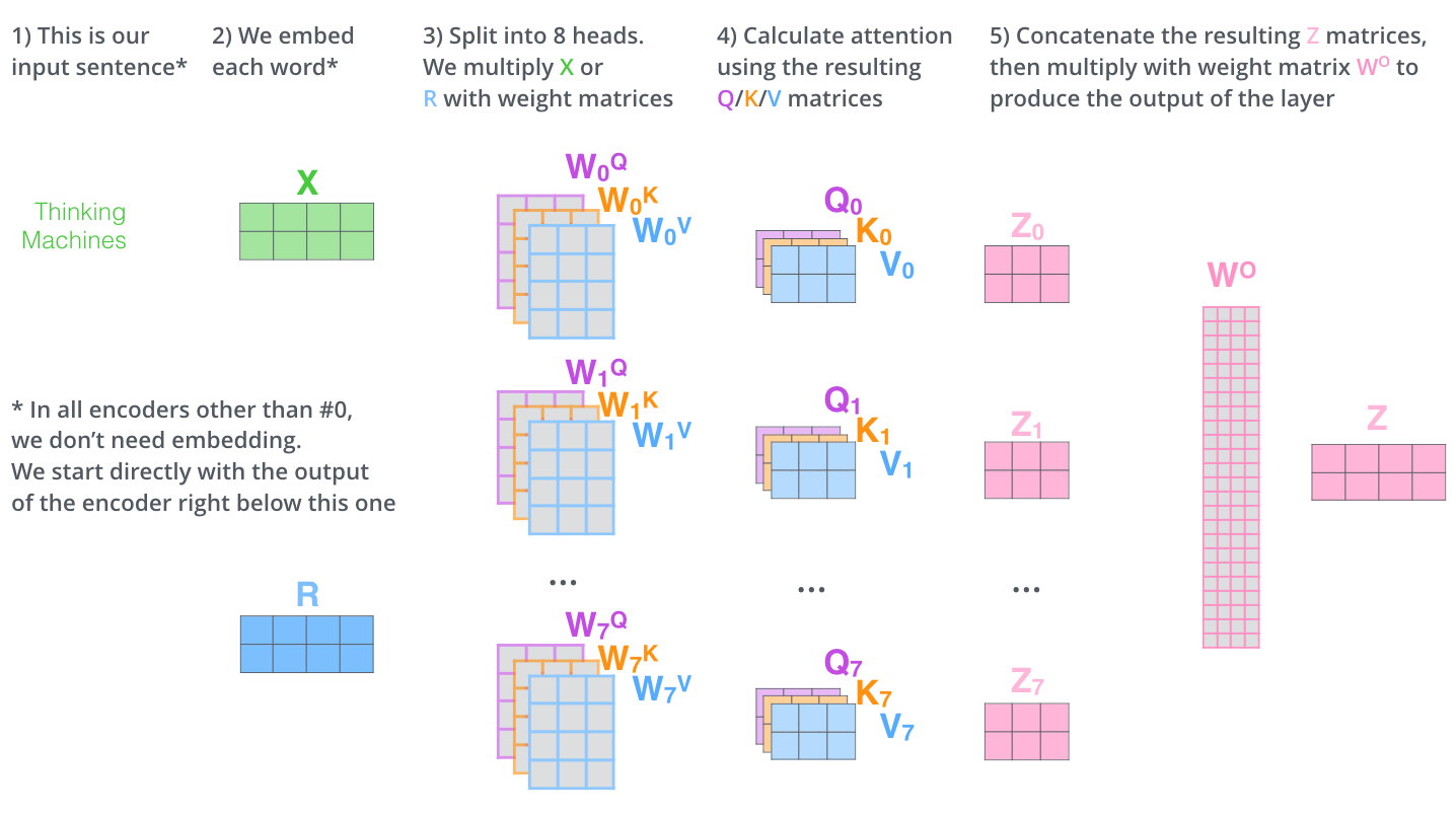
 由于原文叠加了多个编码器（encoder），所以只有第一个使用embedding向量X，其他的使用的是上一个编码器的输出，即上图的R。

可视化两个注意力head的结果，其中一个将‘it’和‘animal’联系在一起，另一个则将‘it’和‘tire’相联系：

 

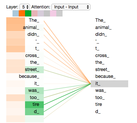
 8个都展示的话就不直观了：

三、位置编码 Positional Encoding

由于在机器翻译中，解码过程是一个顺序操作的过程，也就是当解码某个特征向量时，我们只能看到其之前的解码结果，论文中把这种情况下的multi-head attention叫做masked multi-head attention。 

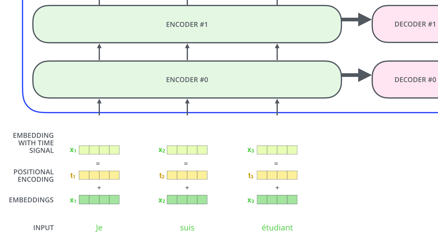
由于本文没有使用RNN、CNN结构处理输入，所以需要额外的手段将数据（字符）之间的位置关系引入网络中。最终采用了下图的方式，利用额外的位置信息编码和原始embedding做点加，输出作为进入网络的原时数据：

 

 

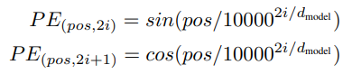
位置信息编码作者选择了正弦曲线，理由是1、公式简单很容易拟合；2、没有额外参数且对输入长度无限制（可以输入比训练集中数据更长的句子）。公式如下：
　　

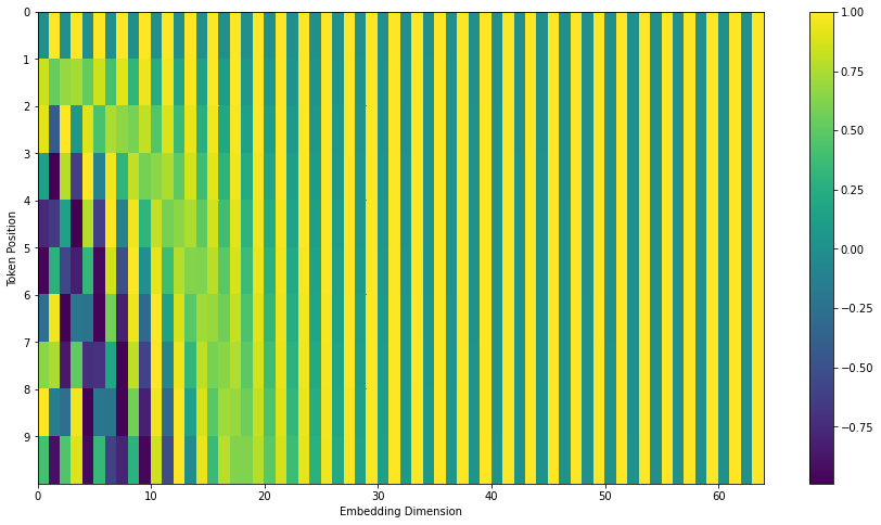
可视化如下，包含10个长度为64的位置编号。条纹状出现是因为奇数和偶数位置的公式不同。

 

 

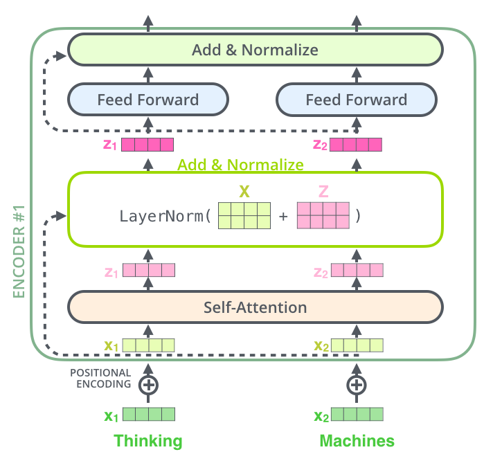
四、残差结构

 作者在每一个block上都使用了2个残差结构：自注意力机制和feed forward两个部分。

 

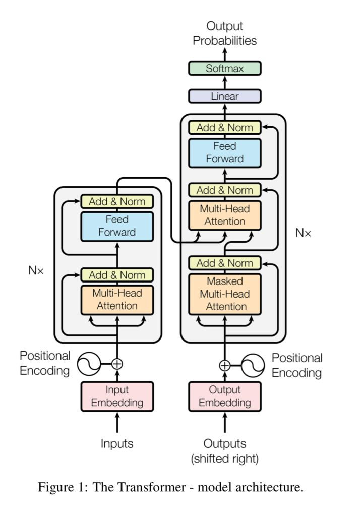
 这里的block包含decode端，实际整个网络类似下面的情况：

 

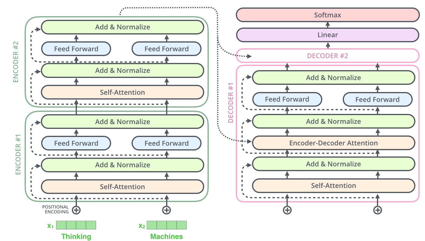
 五、解码器

解码block相对于编码block多了encoder-decoder attention层。

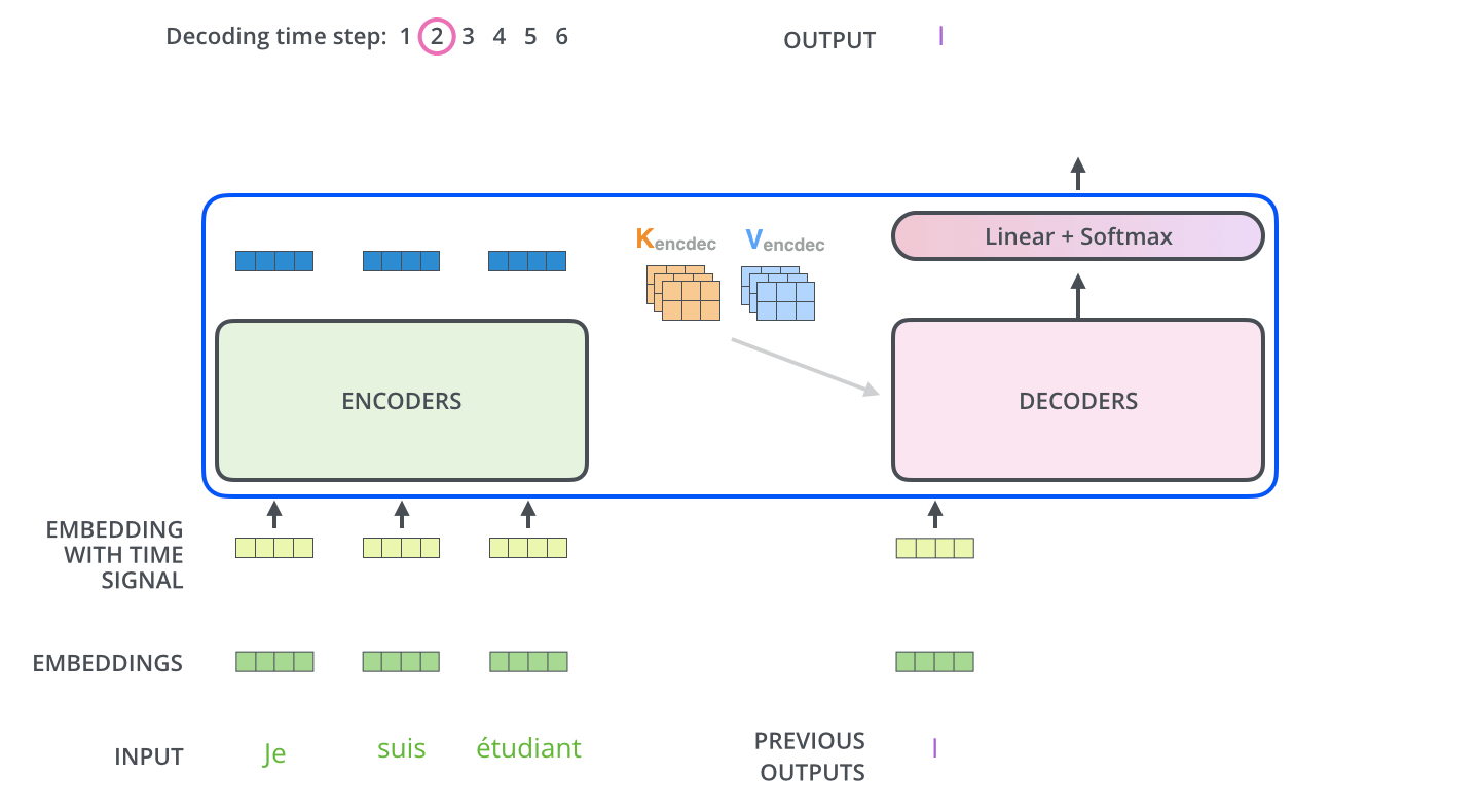
上图中已经可以看到解码部分的结构了：最后一层的encode输出k、v两个向量用于每一个解码block中的encoder-decoder attention计算，每个step中decoder输入一个字符：

1、和前面的词（前面step生成的词）做self attention

2、和encoder输出的每一个词的k、v做encoder-decoder attention

3、完成其他计算，输出本step的词

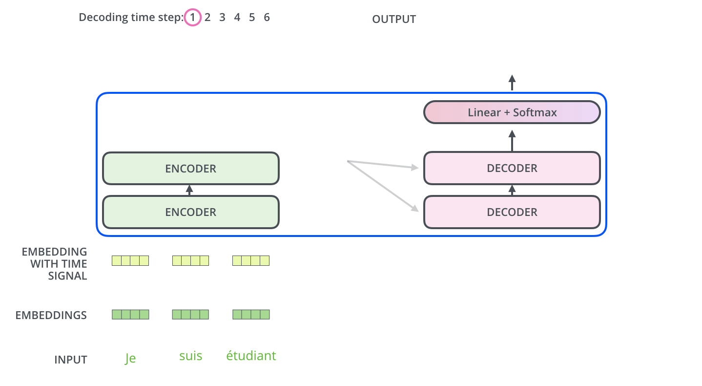
Decoder端每个step输入为上个step输出，初始输入为句子起始符，流程类似下面两图：

 

 

 

 

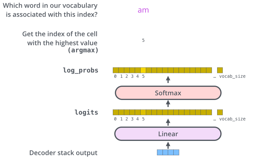
六、Decoder输出处理

 The decoder stack outputs a vector of floats. How do we turn that into a word? That’s the job of the final Linear layer which is followed by a Softmax Layer.

以前没怎么看过nlp的东西，感觉挺神奇的，输出完全是一个one hot的编码，也就是这种特征提取网络其实对动辄尺寸超大的词汇表表达能力很出众，最终一个很正常的分类器就可以完成划分。

 七、原论文补充

复杂度

 

 

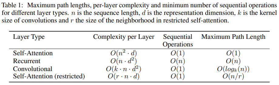
原文中提到为了降低复杂度，可以限制每一个词仅关注附近r个词的相关性，即上表最后一行。

不过这几个复杂度公式没搞明白怎么算的……，推测如下：

SA：n个step，每个step上输入d维向量，输出n维注意力向量

RNN：n个step，每个step上输入d维输出d维，全连接层

卷积：n*d的输入，k*d的卷积核，输出维度仍为n*d

正则化

训练中作者使用了3种正则化方法：

1、作者在每一个layer norm前的add节点前了dropout；

2、作者在endoer和decoder的位置编码add节点后添加dropout；

3、做了训练阶段的标签平滑。

原论文网络结构图