Tensorflow2.0学习-过拟合欠拟合 (四)

文章目录

• 过拟合欠拟合
• • 引包
  • 数据准备
  • 模型准备
  • 跑起来
  • 整体代码

过拟合欠拟合

来看看Tensorflow对于过拟合欠拟合问题是如何解决的，官网是做了一个例子来证明过拟合欠拟合的解决方案的，探索了几种正则化技术。Overfit and underfit

引包

import tensorflow as tf

from tensorflow.keras import layers
from tensorflow.keras import regularizers

print(tf.__version__)

!pip install git+https://github.com/tensorflow/docs

import tensorflow_docs as tfdocs
import tensorflow_docs.modeling
import tensorflow_docs.plots

from  IPython import display
from matplotlib import pyplot as plt

import numpy as np

import pathlib
import shutil
import tempfile

logdir = pathlib.Path(tempfile.mkdtemp())/"tensorboard_logs"
shutil.rmtree(logdir, ignore_errors=True)

数据准备

希格斯数据集，它包含 11,000,000 个示例，每个示例具有 28 个特征和一个二进制类标签。
就发现特别喜欢用.map函数，把方法名做参数传进去，应该是比循环要好用吧。

使用该Dataset.cache方法保证loader不需要在每个epoch重新从文件中读取数据.
在进行批处理之前，还记得在训练集上使用Dataset.shuffle和Dataset.repeat

具体任务就是采用28个特征去预测一个标签。

gz = tf.keras.utils.get_file('HIGGS.csv.gz', 'http://mlphysics.ics.uci.edu/data/higgs/HIGGS.csv.gz')

FEATURES = 28
# 直接读出来
ds = tf.data.experimental.CsvDataset(gz,[float(),]*(FEATURES+1), compression_type="GZIP")

def pack_row(*row):
  label = row[0]
  features = tf.stack(row[1:],1)
  return features, label

packed_ds = ds.batch(10000).map(pack_row).unbatch()

for features,label in packed_ds.batch(1000).take(1):
 	print(features[0])
  	plt.hist(features.numpy().flatten(), bins = 101)
plt.show()

N_VALIDATION = int(1e3)
N_TRAIN = int(1e4)
BUFFER_SIZE = int(1e4)
BATCH_SIZE = 500
STEPS_PER_EPOCH = N_TRAIN//BATCH_SIZE

validate_ds = packed_ds.take(N_VALIDATION).cache()
train_ds = packed_ds.skip(N_VALIDATION).take(N_TRAIN).cache()

validate_ds = validate_ds.batch(BATCH_SIZE)
train_ds = train_ds.shuffle(BUFFER_SIZE).repeat().batch(BATCH_SIZE)

模型准备

过拟合验证
用tf.keras.optimizers.schedules随时间降低学习率。
tf.keras.optimizers.schedules.InverseTimeDecay定义如下：

tf.keras.optimizers.schedules.InverseTimeDecay(
    initial_learning_rate,  # 初始学习率
    decay_steps,  # 多少步降低一次学习率
    decay_rate,  # 降低速率
    staircase=False, # 是否在离散的楼梯中应用衰减
    name=None  # 命名
)

# 公式是这样的
def decayed_learning_rate(step):
  return initial_learning_rate / (1 + decay_rate * step / decay_step)
# 如果staircase是True
def decayed_learning_rate(step):
  return initial_learning_rate / (1 + decay_rate * step / decay_step)

这个例子里学习率和优化器的定义。

lr_schedule = tf.keras.optimizers.schedules.InverseTimeDecay(
  0.001,
  decay_steps=STEPS_PER_EPOCH*1000,
  decay_rate=1,
  staircase=False)

def get_optimizer():
  return tf.keras.optimizers.Adam(lr_schedule)

# 查看学习率变化曲线
step = np.linspace(0,100000)
lr = lr_schedule(step)
plt.figure(figsize = (8,6))
plt.plot(step/STEPS_PER_EPOCH, lr)
plt.ylim([0,max(plt.ylim())])
plt.xlabel('Epoch')
_ = plt.ylabel('Learning Rate')
plt.show()

再用一个回调函数来打印训练的信息，回调的话，看作一个异步操作就好，就是训练做训练的，训练过程的一些参数调整，打印信息什么的，交给回调函数去做，而且还不影响训练。这里用了一个tf.keras.callbacks.EarlyStopping函数，可以在合适的位置让训练停下来。
函数定义如下：

tf.keras.callbacks.EarlyStopping(
    monitor='val_loss',  # 要监控的数值名称
    min_delta=0,  # 被监测数量的最小变化被认为是改进，即小于 min_delta 的绝对变化，将被视为没有改进
    patience=0,  # 如果在patience个epoch没有改善的话，就停止。
    verbose=0,  # 输出信息的模式
    mode='auto', # {"auto", "min", "max"} min 如果被检测的数值停止减少训练就停止，max 停止增长训练就停止，auto 根据被检测的数值名称自动判断
    baseline=None,  # 监控数量的基线值。如果模型没有显示出对基线的改进，则训练将停止。
    restore_best_weights=False  # 是否采用最佳表现的权重，若不是，就是停止时的权重
)

tf.keras.callbacks.TensorBoard就是一个记录训练信息的函数，可以在网页中查看，
在这个例子中回调函数有打印训练进度，早停，记录训练信息。

tfdocs.modeling.EpochDots()就是进度，一个点表示训练一次，训练一百次就打印信息。（不如tqdm来的方便）

def get_callbacks(name):
  return [
    tfdocs.modeling.EpochDots(),
    tf.keras.callbacks.EarlyStopping(monitor='val_binary_crossentropy', patience=200),
    tf.keras.callbacks.TensorBoard(logdir/name),
  ]

还是用model.compile来设置损失函数、优化器以及训练信息。model.fit就是开训，这里都集成在一个方法中。

def compile_and_fit(model, name, optimizer=None, max_epochs=10000):
  if optimizer is None:
    optimizer = get_optimizer()
  model.compile(optimizer=optimizer,
                loss=tf.keras.losses.BinaryCrossentropy(from_logits=True),
                metrics=[
                  tf.keras.losses.BinaryCrossentropy(
                      from_logits=True, name='binary_crossentropy'),
                  'accuracy'])

  model.summary()

  history = model.fit(
    train_ds,
    steps_per_epoch = STEPS_PER_EPOCH,
    epochs=max_epochs,
    validation_data=validate_ds,
    callbacks=get_callbacks(name),
    verbose=0)
  return history

跑起来

好了到了检验不同模型拟合程度比较了，先来个简单的两层全连接

tiny_model = tf.keras.Sequential([
    layers.Dense(16, activation='elu', input_shape=(FEATURES,)),
    layers.Dense(1)
])
#  定义个字典
size_histories = {}
#  结果存放
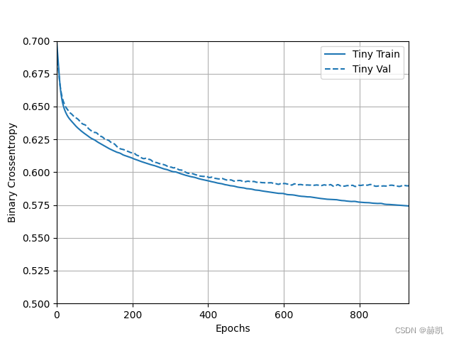
size_histories['Tiny'] = compile_and_fit(tiny_model, 'sizes/Tiny')
#  跑完之后看看图
plotter = tfdocs.plots.HistoryPlotter(metric = 'binary_crossentropy', smoothing_std=10)
plotter.plot(size_histories)
plt.ylim([0.5, 0.7])
plt.show()

依次再试试稍微复杂模型

small_model = tf.keras.Sequential([
    # `input_shape` is only required here so that `.summary` works.
    layers.Dense(16, activation='elu', input_shape=(FEATURES,)),
    layers.Dense(16, activation='elu'),
    layers.Dense(1)
])
size_histories['Small'] = compile_and_fit(small_model, 'sizes/Small')

medium_model = tf.keras.Sequential([
    layers.Dense(64, activation='elu', input_shape=(FEATURES,)),
    layers.Dense(64, activation='elu'),
    layers.Dense(64, activation='elu'),
    layers.Dense(1)
])
size_histories['Medium']  = compile_and_fit(medium_model, "sizes/Medium")

large_model = tf.keras.Sequential([
    layers.Dense(512, activation='elu', input_shape=(FEATURES,)),
    layers.Dense(512, activation='elu'),
    layers.Dense(512, activation='elu'),
    layers.Dense(512, activation='elu'),
    layers.Dense(1)
])
size_histories['large'] = compile_and_fit(large_model, "sizes/large")

# 最后看看结果
plotter.plot(size_histories)
a = plt.xscale('log')
plt.xlim([5, max(plt.xlim())])
plt.ylim([0.5, 0.7])
plt.xlabel("Epochs [Log Scale]")
plt.show()

不得不说Tensorflow还真的是简单，画图什么的都自动完成了。从图里明显看出来，模型越复杂对于训练数据集真效果真不错，但是对于验证集的就不好了，就是过拟合了。

整体代码

import tensorflow as tf

from tensorflow.keras import layers
from tensorflow.keras import regularizers

print(tf.__version__)

import tensorflow_docs as tfdocs
import tensorflow_docs.modeling
import tensorflow_docs.plots

from IPython import display
from matplotlib import pyplot as plt

import numpy as np

import pathlib
import shutil
import tempfile

logdir = "E:/tensorflow2.0/tensorboard_logs/"
shutil.rmtree(logdir, ignore_errors=True)

gz = tf.keras.utils.get_file('HIGGS.csv.gz', 'http://mlphysics.ics.uci.edu/data/higgs/HIGGS.csv.gz')

FEATURES = 28
# 直接读出来
ds = tf.data.experimental.CsvDataset(gz, [float(), ] * (FEATURES + 1), compression_type="GZIP")


def pack_row(*row):
    label = row[0]
    features = tf.stack(row[1:], 1)
    return features, label


packed_ds = ds.batch(10000).map(pack_row).unbatch()

# for features, label in packed_ds.batch(1000).take(1):
#     print(features[0])
#     plt.hist(features.numpy().flatten(), bins=101)
# plt.show()

N_VALIDATION = int(1e3)
N_TRAIN = int(1e4)
BUFFER_SIZE = int(1e4)
BATCH_SIZE = 500
STEPS_PER_EPOCH = N_TRAIN // BATCH_SIZE

validate_ds = packed_ds.take(N_VALIDATION).cache()
train_ds = packed_ds.skip(N_VALIDATION).take(N_TRAIN).cache()

validate_ds = validate_ds.batch(BATCH_SIZE)
train_ds = train_ds.shuffle(BUFFER_SIZE).repeat().batch(BATCH_SIZE)

lr_schedule = tf.keras.optimizers.schedules.InverseTimeDecay(
    0.001,
    decay_steps=STEPS_PER_EPOCH * 1000,
    decay_rate=1,
    staircase=False)


def get_optimizer():
    return tf.keras.optimizers.Adam(lr_schedule)


step = np.linspace(0, 100000)


# lr = lr_schedule(step)
# plt.figure(figsize=(8, 6))
# plt.plot(step / STEPS_PER_EPOCH, lr)
# plt.ylim([0, max(plt.ylim())])
# plt.xlabel('Epoch')
# _ = plt.ylabel('Learning Rate')
# plt.show()

def get_callbacks(name):
    return [
        tfdocs.modeling.EpochDots(),
        tf.keras.callbacks.EarlyStopping(monitor='val_binary_crossentropy', patience=200),
        tf.keras.callbacks.TensorBoard(logdir+name),
    ]


def compile_and_fit(model, name, optimizer=None, max_epochs=10000):
    if optimizer is None:
        optimizer = get_optimizer()
    model.compile(optimizer=optimizer,
                  loss=tf.keras.losses.BinaryCrossentropy(from_logits=True),
                  metrics=[
                      tf.keras.losses.BinaryCrossentropy(
                          from_logits=True, name='binary_crossentropy'),
                      'accuracy'])

    model.summary()

    history = model.fit(
        train_ds,
        steps_per_epoch=STEPS_PER_EPOCH,
        epochs=max_epochs,
        validation_data=validate_ds,
        callbacks=get_callbacks(name),
        verbose=0)
    return history


tiny_model = tf.keras.Sequential([
    layers.Dense(16, activation='elu', input_shape=(FEATURES,)),
    layers.Dense(1)
])

size_histories = {}

size_histories['Tiny'] = compile_and_fit(tiny_model, 'sizes/Tiny')

plotter = tfdocs.plots.HistoryPlotter(metric='binary_crossentropy', smoothing_std=10)
plotter.plot(size_histories)
plt.ylim([0.5, 0.7])
plt.show()
small_model = tf.keras.Sequential([
    # `input_shape` is only required here so that `.summary` works.
    layers.Dense(16, activation='elu', input_shape=(FEATURES,)),
    layers.Dense(16, activation='elu'),
    layers.Dense(1)
])
size_histories['Small'] = compile_and_fit(small_model, 'sizes/Small')

medium_model = tf.keras.Sequential([
    layers.Dense(64, activation='elu', input_shape=(FEATURES,)),
    layers.Dense(64, activation='elu'),
    layers.Dense(64, activation='elu'),
    layers.Dense(1)
])
size_histories['Medium']  = compile_and_fit(medium_model, "sizes/Medium")

large_model = tf.keras.Sequential([
    layers.Dense(512, activation='elu', input_shape=(FEATURES,)),
    layers.Dense(512, activation='elu'),
    layers.Dense(512, activation='elu'),
    layers.Dense(512, activation='elu'),
    layers.Dense(1)
])
size_histories['large'] = compile_and_fit(large_model, "sizes/large")

# 最后看看结果
plotter.plot(size_histories)
a = plt.xscale('log')
plt.xlim([5, max(plt.xlim())])
plt.ylim([0.5, 0.7])
plt.xlabel("Epochs [Log Scale]")
plt.show()